Projected climate variability of internal waves in the andaman sea

ABSTRACT The Andaman Sea, in the northeast Indian Ocean, is renowned for large-amplitude internal waves. Here, we use a global climate model (CanESM5) to investigate the long-term

variability of internal waves in the Andaman Sea under a range of shared socioeconomic pathway (SSP) scenarios. SSPs are future societal development pathways related to emissions and land

use scenarios. We project that mean values of depth-averaged stratification will increase by approximately 6% (SSP1-2.6), 7% (SSP2-4.5), and 12% (SSP5-8.5) between 1871-1900 and 2081-2100.

Simulating changes in internal tides between the present (2015-2024) and the end-century (2091-2100), we find that the increase in stratification will enhance internal tide generation by

approximately 4 to 8%. We project that the propagation of internal tides into the Andaman Sea and the Bay of Bengal will increase by 8 to 18% and 4 to 19%, respectively, under different SSP

scenarios. Such changes in internal tides under global warming will have implications for primary production and ecosystem health not only in the Andaman Sea but also in the Bay of Bengal.

SIMILAR CONTENT BEING VIEWED BY OTHERS INTERANNUAL VARIABILITY OF INTERNAL TIDES IN THE ANDAMAN SEA: AN EFFECT OF INDIAN OCEAN DIPOLE Article Open access 30 June 2022 SEA LEVEL EXTREMES AND

COMPOUNDING MARINE HEATWAVES IN COASTAL INDONESIA Article Open access 27 October 2022 ENHANCED GENERATION OF INTERNAL TIDES UNDER GLOBAL WARMING Article Open access 03 September 2024

INTRODUCTION The vertical distribution of temperature, salinity, and pressure determines ocean stratification. In light of human-induced climate change significantly altering oceanic

temperature and salinity distribution, it is expected that oceanic stratification will be affected1,2. Global ocean stratification has increased by 0.9% per decade during 1960–20183. The

majority of the increase (71%) occurred in the upper 200 m of the ocean and was primarily caused by temperature changes, with salinity changes playing a minor role locally3. Internal waves

(IWs) form when perturbations in the stratified layer induce them to move up or down, and these perturbations encounter a restoring buoyancy force4. Internal tides (ITs) are IWs that

oscillate at tidal frequencies. The vertical transfer of water, heat and other climatically relevant tracers in the ocean is driven by turbulent mixing from breaking oceanic IWs. As a

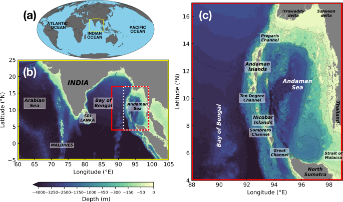
result, IWs play a crucial role in controlling the movement and distribution of heat and carbon across the climate system5,6. The Andaman Sea is located on the northeastern side of the

Indian Ocean (Fig. 1a, b), bordered on the west by an arc of islands stretching from northern Sumatra to the Irrawaddy delta (Fig. 1c). The monsoonal climate dominates the region, with the

northeast or winter monsoon prevailing from December to March and the southwest or summer monsoon prevalent from June to September7. It receives a large volume of freshwater influx from the

Irrawaddy and Salween rivers in the northern part8. Equatorial forcing dominates the mean coastal circulation in the Andaman Sea9,10. It is also characterised by extraordinarily

large-amplitude IWs11,12. Semidiurnal ITs are the most energetic part of the entire IW spectrum in the Andaman Sea13,14,15,16. Yadidya et al.16 suggested strong IT seasonal and spatial

variability using in-situ observations and numerical model simulations. Moreover, the changes in stratification due to the effect of the Indian Ocean Dipole (IOD) modulates the interannual

variability of IWs in this region17. The Andaman Sea’s coral reefs have been regarded as being among the most diversified and vast in the Indian Ocean18. Roder et al.19 reported that

IWs-exposed corals are more heterotrophic and rich in nutrient concentrations. Nielsen et al.20 observed maximum _C__h__l_ _a_ and primary production where the pycnocline interacted with

bottom topography. This interaction helped in sub-surface nutrient-rich water mixing with the surface layers suggesting that IWs can enhance primary and secondary productivity. We used

CanESM5 from CMIP6 model simulations (see ‘Methods’) to examine the long-term variability of IW activity in Historical (1850–2014) and future (2015–2100) scenarios, given the huge

consequences that IWs can have on the bio-physical ecosystem of the Andaman Sea. Density stratification is used as a proxy for IW activity21,22 to quantify its long-term changes (see

‘Methods’). We assess the impact of temperature and salinity on density stratification because both of them affect density16,17. One of the most severe hazards to coral reefs caused by

climate change is the increasing frequency of severe coral bleaching23. Wyatt et al.24 hypothesised that the effect of IWs on coral reefs could establish and sustain thermal refuges where

heat stress and coral bleaching risk can be controlled. However, future implications will depend on how the IW climate responds to further warming and increasing ocean stratification.

Therefore, numerical model simulations are used to estimate changes in the IT energetics between the present (2015–2024) and end-century (2091–2100) with changing stratification. Later, we

also discuss their implications on the bio-physical environment. RESULTS CHANGES IN STRATIFICATION The long-term changes in the density stratification are evaluated based on the

stratification anomalies computed with respect to the density stratification in the Historical simulations (Fig. 2a). Since 1850, the Andaman Sea’s annual density stratification did not show

any long-term variability until 2000. However, it has increased by 0.2 cph from 2000 to 2014 in the Historical. The future projections under different scenarios also indicate an increasing

trend with stratification increasing by 0.9 cph by the end-century under SSP5-8.5, which is the highest emissions no-policy baseline scenario. The Historical simulation’s annual cycle of

stratification profiles shows a bimodal signal with maximum stratification near 70–90 m (Fig. 2b). Strong positive (negative) anomalies are seen from 25 to 60 m (90–120 m), especially during

boreal autumn and winter months, in all the SSP scenarios (Fig. 2c–e). This indicates a strong increase (decrease) in the stratification of the near-surface (sub-surface) waters in the

coming years. Furthermore, we investigated the relative contributions of variations in temperature and salinity to the trend in density stratification profiles on annual and seasonal

timescales (Fig. 3). The corresponding profiles of salinity and temperature trends are shown in Fig. 4. A three-layered trend pattern can be seen in the vertical (0–200 m), with a layer of

decreasing trend sandwiched between two layers of an increasing trend in all the simulations. In the Historical (Fig. 3a), the first layer of increasing trend is seen up to 85 m, with the

maximum (0.34 ± 0.14 cph/century) at 65 m. The layer of decreasing trend is present below that up to 185 m, with the maximum (-0.48 ± 0.12 cph/century) at 125 m. Increasing salinity (Fig. 

4a) from 1850 to 2014 until 150 m resulted in salinity contributing to decreasing stratification trend (Fig. 3a). The effect of temperature is present throughout the water column, with

temperature increasing from the surface to 70 m and below 125 m (Fig. 4e). Contrarily, salinity showed a decreasing trend from surface to 85 m in SSP1-2.6 (Fig. 4b), which resulted in

salinity influencing a strong increasing trend in stratification (Fig. 3b). In fact, the salinity effect dominates the first layer until 75 m, where a uniform increase in temperature is

noticed (Fig. 4f). The temperature effect is present below 75 m leading to a decreasing trend up to 150 m. In the case of SSP2-4.5 (Fig. 3c), the impact of temperature and salinity in the

near-surface layers is exactly the opposite. This has resulted in the shallowest increasing trend layer present only in the top 50 m. A thick layer of decreasing trend is observed from 50 to

150 m. A strong increase in both temperature (Fig. 4g) and salinity (Fig. 4c) in the near-surface layers has caused this to happen. In the extreme scenario of SSP5-8.5 (Fig. 3d), the

stratification, fuelled by both temperature and salinity changes, is increasing from surface to 70 m, with the maximum increase (3.8 ± 0.65 cph/century) at 40 m. The decreasing trend layer

is present from 70 to 140 m, below which the stratification increased strongly again. In boreal winter, the Andaman Sea experiences the northeast monsoon associated with relatively strong

precipitation and cooler temperatures near the surface, resulting in temperature inversions7. The vertical profiles of trends in Historical (Fig. 3e) and in all SSP scenarios (Fig. 3f–h)

follow a similar pattern to that of annual (Fig. 3a–d). A strong decreasing trend in precipitation flux (Supplementary Fig. 1a) and water flux (Supplementary Fig. 1e) are observed in

Historical, which could be contributing to increased salinity in the near-surface layers. The Andaman Sea receives maximum insolation and net heat flux during spring (April and May). This

results in the formation of the seasonal thermocline and shallow isothermal layer depth7. The maximum of the first layer of increasing trend (Fig. 3i–l) is very shallow compared to the

annual (Fig. 3a–d). For example, in the Historical, it (0.25 ± 0.32  cph/century) is seen at 25 m during spring but is at 65 m in annual. Moreover, there is a strong decreasing trend in

water flux (Supplementary Fig. 1e–h) in all the experiments except SSP1-2.6 indicating excessive evaporation leading to high salinity in the near-surface waters. Therefore salinity effect

shows a decreasing trend in stratification except in SSP1-2.6. The onset of the southwest monsoon characterises the boreal summer season7. The precipitation flux (Supplementary Fig. 1a–d)

and water flux (Supplementary Fig. 1e–h) showed the least variability among all seasons except in SSP1-2.6, where both showed an increasing trend. The salinity trend (Fig. 4a–d) is closest

to the annual trend, whereas the temperature (Fig. 4e–h) showed the maximum increasing trend in the near-surface (up to 75 m). Regarding the trend in stratification (Fig. 3m–p), the

Historical trend showed a four-layer pattern with an additional decreasing trend near the surface. This is caused due to uniform increase in temperature until 50 m and a strong decreasing

trend effect by salinity. The maximum (4.9 ± 0.81 cph/century) of the increasing trend in the near-surface is the second-highest among all the seasons in SSP5-8.5. During autumn, the

northern part of the Andaman Sea receives a massive amount of freshwater influx from the Irrawaddy and Salween rivers8. The trend in water flux (Supplementary Fig. 1e–h) shows that the river

runoff has increased in the Historical and is expected to increase in SSP2-4.5 and SSP5-8.5 scenarios. Furthermore, the precipitation flux (Supplementary Fig. 1a–d) shows a strong

increasing trend in SSP2-4.5 and SSP5-8.5. The effect of this can be seen in the salinity trends (Fig. 4a–d), where the lowest increasing trend is seen in Historical and SSP2-4.5; and the

largest decreasing trend in SSP1-2.6 and SSP2-4.5. The effect of both temperature and salinity results in the highest increasing trend (maximum of 0.83 ± 0.36, 2.25 ± 1.37, 1.1 ± 1.52, 5.54 

± 1.13  cph/century) in the first layer of near-surface waters in all the experiments (Historical, SSP1-2.6, SSP2-4.5, SSP5-8.5) (Fig. 3q–t). This shows that the increasing trend in

stratification is highest during autumn and will continue to be during the same season in the future as well. In summary, the density stratification trend profile shows a three-layer

structure in the upper 200 m, with two layers of increasing trend separated by a layer of decreasing trend. It showed significant seasonal variability due to the combined effect of

temperature and salinity. Under SSP1-2.6, in which the long-term estimate is projected to increase global warming by 1.8 °C25, the stratification increase is caused by salinity changes with

no net effect from temperature changes. Contrarily, the salinity changes induced a negative effect on increasing stratification, which is completely fuelled by the temperature changes in

SSP2-4.5 (long-term estimate of an increase by 2.7 °C25). In the high-end scenario of SSP5-8.5, where an increase of 4.4 °C is expected by 210025, both temperature and salinity changes are

contributing to the stratification increase. The depth-averaged stratification shows an increasing trend of 0.014 ± 0.04, 0.21 ± 0.12, 0.06 ± 0.11, and 0.73 ± 0.11 cph/century under

Historical (1850–2014), SSP1-2.6, SSP2-4.5, and SSP5-8.5 scenarios (2015–2100), respectively. The time series of density stratification profiles shown in Supplementary Fig. 2 reveals the

same. For instance, in the Historical, the maximum buoyancy frequency was mostly less than 14 cph at 75 m. Whereas in SSP5-8.5, it is exceeding 16 cph at 45 m. The upwelling of highly

stratified layers is also clearly seen in all the SSP scenarios. COMPARISON OF BAROCLINIC TIDAL ENERGY BUDGET BETWEEN THE PRESENT AND FUTURE This section considers the mean stratification

from 2015 to 2024 in SSP1-2.6 as the ‘present’ stratification. On the other hand, the mean stratification from 2091 to 2100 is considered as the ‘end-century’ stratification and is taken for

SSP1-2.6, SSP2-4.5 and SSP5-8.5 scenarios. These two time periods are selected to evaluate and quantify the effect of increasing stratification from the present decade to the final decade

in the CMIP6 (CanESM5) simulations on the IT energy budget. The temperature and salinity profiles and the corresponding density stratification used for model initialisation are shown in Fig.

 5. In the present SSP1-2.6, the buoyancy frequency increased until 75 m and gradually decreased below this depth. In different SSP scenarios, the end-century stratification is higher in the

near-surface layers but is less than the present from 70–80 to 150–160 m. The changes in the IT energy budget (see 'Methods') comprising of IT generation, propagation, and

dissipation from the present to the end-century are discussed in detail (Fig. 6). Six sub-regions (Fig. 6a) are selected for this analysis where the IT generation is relatively high16,17. In

the Preparis Channel (PC), located in the northwestern Andaman Sea, the IT generation changed very little in the SSP1-2.6 (Fig. 6b, c) and SSP2-4.5 (Fig. 6b, d) scenarios but increased by

9% in SSP5-8.5 (Fig. 6b, e). However, the westward propagation of IT into the Bay of Bengal and eastward propagation into the Andaman Sea is seen to increase by 1.2–17.5% and 8–16.2% in

different scenarios. The baroclinic energy conversion in the Ten Degree Channel (TDC), located between the Andaman and Nicobar Islands, could increase by 2.9–9.2%. The local dissipation

ratio in present is 0.53 (Fig. 6b) but is projected to decrease by 17.3–25.1% (Fig. 6c–e). The decrease in dissipation could result in increased baroclinic flux into both Bay of Bengal and

the Andaman Sea, but more so into the latter by 19–33.9% (Fig. 6c–e). Sombrero Channel (SC) is the main generation site for IT in the Andaman Sea. The IT generation is found to be almost the

same in the SSP1-2.6 (Fig. 6b, c) and SSP2-4.5 (Fig. 6b, d) scenarios but could decrease by 6.7% in SSP5-8.5 (Fig. 6b, e). The propagation of IT also showed the least amount of variability

in the SSP1-2.6 and SSP2-4.5 but could increase by 4.9% and 12.6% in the Bay of Bengal and Andaman Sea in SSP5-8.5, respectively. However, the local dissipation ratio could decrease by

9.6–62.3% (Fig. 6c–e) from 0.15 (Fig. 6b). The Great Channel (GC) is the southernmost channel between the Nicobar Islands and North Sumatra. The barotropic to baroclinic energy conversion is

predicted to increase by 13.8–24.2%. The local dissipation efficiency ratio increased by 27.2% (Fig. 6c) and 13.2% (Fig. 6d) but decreased by 21.3% (Fig. 6e) from 0.24 (Fig. 6b) in

SSP1-2.6, SSP2-4.5, and SSP5-8.5, respectively. This increased the IT propagation into the Bay of Bengal by 17.5–91%. The generation of IT in the North East Andaman Sea (NEAS) increased by

4.1–10.1%. However, a massive increase is seen in the IT propagating into NEAS by 68.9–98% from the western side. This is mainly due to the increased baroclinic flux into the Andaman Sea at

PC, TDC, and SC. The local dissipation ratio also increases from 0.95 (Fig. 6b) to 1.1–1.45 (Fig. 6c–e), an increase of 15.3–52.6%. The ratio >1 indicates remote dissipation of IT. In the

South East Andaman Sea (SEAS) region, which connects the Andaman Sea to the Malacca Strait, the IT generation increased by 31.9% in SSP5-8.5 (Fig. 6e) but is relatively similar in the other

two scenarios (Fig. 6c, d). On the other hand, the local dissipation efficiency increased from 0.81 to 0.88–0.93 (8.6–15%). The model simulations suggest that the amount of IT generated is

increasing in most of the generation sites with changing stratification. The mean energy conversion of the six main generation sites increased by 4.4%, 4.05%, and 7.66% under SSP1-2.6,

SSP2-4.5, and SSP5-8.5 scenarios, respectively. The local dissipation in the western Andaman Sea is also decreasing significantly. Therefore, a sharp increase in the baroclinic energy flux

into the Bay of Bengal (4.19–19.25%); and into the Andaman Sea (7.95–18.05%) is noticed. Consequently, the eastern Andaman Sea is receiving high IT flux resulting in high remote dissipation

of IT. DISCUSSION AND CONCLUSIONS IW activity in the Andaman Sea has been influenced by changes in density stratification caused due to climate change and has increased since the turn of the

century. Under future SSP scenarios, changes in temperature and salinity result in increased density stratification, especially in the near-surface waters where the euphotic zone exists.

Boreal autumn is expected to see the maximum increase in stratification when the IOD’s effect is maximum. The Andaman Sea is quite distinct from other regions like South China Sea, where

large-amplitude IWs are present. It is unique due to the presence of a double pycnocline, where the stratification of density is affected by both temperature and salinity16,17,26. Li et al.3

reported that during 1960–2018, > 90% of the increase in stratification is caused by temperature changes in the global oceans. However, in the Andaman Sea, we found that salinity changes

are also important along with temperature changes in both Historical and future SSP scenarios. For example, increasing salinity of the near-surface waters in SSP2-4.5, with intermediate

greenhouse gas emissions, leads to a negative effect on the increasing stratification from 2015 to 2100. Whereas in the other two scenarios, i.e., SSP1-2.6 and SSP5-8.5, which are on either

end of the spectrum in terms of emissions, decreasing salinity has a positive effect on the increasing stratification. The signal-to-noise ratio between different realisations of CanESM5 in

Supplementary Fig. 3 also shows that the uncertainty in salinity changes is high within the top 30 m in all the SSP scenarios. However, the mechanisms for the differences in salinity changes

between the SSP scenarios are beyond the scope of this study but could be due to changes in the river runoff, precipitation, evaporation, and the dynamical processes related to them. Even

though the effect of salinity and temperature changes is different between different SSP scenarios, their cumulative effect has resulted in increasing stratification in all the cases.

Therefore, we carried out model simulations using MITgcm to quantify and evaluate the changes in IT energy budget between the first and last decades of SSP simulations. We assumed that the

first decade (2015–2024) is best represented by the SSP1-2.6, which is the low end of the range of potential future pathways, and considered the mean stratification to represent the

‘present’. Later, we compared the results from the ‘present’ to ‘end-century’ (2091–2100) of all the three SSP scenarios consisting of the low end (SSP1-2.6), the medium part (SSP2-4.5), and

the high end (SSP5-8.5) of the range of future pathways in terms of emissions and global temperature rise27. The model simulations suggested a significant increase in the IT generation and

propagation into the Andaman Sea by the end-century. The increase in IT generation and associated dissipation can influence the large-scale ocean circulation in the northern Indian Ocean28.

The resultant changes in the IW field could play a significant, though underappreciated, role in increasing primary productivity; and protecting diverse coral reefs. Increasing diapycnal

mixing as a result of increased dissipation rates would boost the supply of nutrients and plankton that aid in the development of coral reef29. Thermal stress in the future SSP scenarios is

three to four times higher than it is now, posing a serious threat to the health of future reef ecosystems30. The increase in the propagation of ITs into the Andaman Sea could provide

much-needed thermal relief to the diverse corals present in this region. By regularly flushing reefs with cooler water, IWs can alter species assemblages31, alleviate thermal stress32, and

lower corals’ vulnerability to bleaching24,33. Recent observations34,35 and modelling studies36 indicated the IWs generated in the Andaman Sea can travel as far as the east coast of India,

Sri Lanka and Maldives. They contribute to vertical mixing near the coasts, where the IWs break and release their energy. The local dissipation in the western Andaman Sea has decreased

significantly in the end-century simulations. Hence, the increase in the baroclinic flux into the Bay of Bengal from PC, TDC, SC and GC can contribute to reducing the thermal stress on

remote coral reefs present in the coastal waters of Maldives, Sri Lanka and the east coast of India. Field measurements in the northern South China Sea revealed that the dissipation of IWs

led to the pumping of nutrients to the oligotrophic surface water, thereby causing a rapid increase of phytoplankton37. The increased dissipation and mixing in the eastern Andaman Sea and

the Bay of Bengal could enhance primary and secondary productivity20,38. Muacho et al.39 also suggested that IWs can increase the amount of carbon uptake, thereby enhancing the primary

production on 3 to 4-day timescales. In addition to boosting marine production through mixing, IWs can directly transfer a large volume of nutrients and chemicals. The schematic diagram

shown in Fig. 7 summarises this study. We found that the salinity and temperature changes play different roles on increasing stratification in different SSP scenarios from 2015 to 2100.

Model simulations showed some interesting results where a significant increase in the IT generation in the Andaman Sea led to an increase in the IT propagation into both the Andaman Sea and

Bay of Bengal. Consequently, the remote dissipation in both the Andaman Sea and Bay of Bengal are projected to increase. Subsequently, we discussed the potential implications of the

increased stratification and IW activity on the vast and diverse coral reefs in the northern Indian Ocean. We also suggest that the enhanced mixing could potentially increase marine

productivity in this region. This study’s results can be a vital tool for coral reef conservation and management in a warming ocean. METHODS DATA SOURCES AND PROCESSING The interannual

variability in the equatorial Indian Ocean is primarily driven by the IOD40, which is a coupled ocean and atmospheric phenomenon. A positive IOD is characterised by warm sea surface

temperature anomalies on the western side of the equatorial Indian Ocean and vice versa on the eastern side. On the other hand, warm waters are present on the eastern side during a negative

IOD event. According to ref. 41, the following CMIP6 models were able to simulate the dynamics of the IOD, which largely influences the Andaman Sea stratification17, reasonably well. They

are CanESM5, IPSL-CM6A-LR, ACCESS-CM2, and GIDD-E2-1-H. The annual cycle of buoyancy stratification of these four global climate models during 1993–2014 is compared with Ocean Reanalysis

System 542 (ORAS5) data in Fig. 8. The root mean square error (RMSE) between the time series of ORAS5 stratification and the four CMIP6 models is also shown. CanESM5 (r1i1p2f1) is the most

accurate in capturing the annual cycle and the depths of maximum stratification among the four models. The vertical profiles of RMSE also show the least error in CanESM5. Maximum RMSE at 25 

m could be due to overestimation of stratification due to seasonal or secondary thermocline during the spring season. The Historical experiment and three Shared Socioeconomic Pathways (SSPs)

scenarios (SSP1-2.6, SSP2-4.5 and SSP5-8.5) are chosen from CanESM5 in this study27. SSP1-2.6 reflects the low end of the range of potential future forcing pathways and updates the RCP2.6

(Representative Concentration Pathway) from CMIP5. It combines low vulnerability, less obstacles for mitigation, and a low forcing signal to create a multi-model mean warming by 2100 that is

predicted to be much less than 2 °C. SSP2-4.5 represents the medium part of the range of future forcing pathways which combines intermediate societal vulnerability and intermediate forcing

level. It is an update of the RCP4.5 pathway. SSP5-8.5 is the high end of the range of future pathways and an update of RCP8.5, which produces a radiative forcing of 8.5 W/m2 in 2100. All

computations and analyses were carried out in Python on the cloud-based computing platform _Pangeo_. This study’s workflow makes use of _xarray_43,44, _dask_45, _xgcm_46, _xmitgcm_47,

_xesmf_48 and _xmip_49. DENSITY STRATIFICATION AND INTERNAL WAVES The generation of IWs (conversion of barotropic tides to baroclinic motions) is directly proportional to _N_2, as shown by

the equation of 'Baines force', _F__B_, in ref. 22 given as $${F}_{B}={N}^{2}{w}_{bt}{\omega }_{bt}^{-1}$$ (1) where _g_ is gravitational acceleration, _ρ_ is density, _ρ_0 is

background density, _z_ is depth, _w__b__t_ is the vertical barotropic velocity, _ω__b__t_ is the barotropic tidal frequency, and _N_ is the Brunt–Väisälä buoyancy frequency given by

$$N=\sqrt{\frac{-g}{{\rho }_{0}}\frac{\partial \rho }{\partial z}}$$ (2) Therefore, increased density stratification in the pycnocline increases IW generation by the barotropic tide.

Numerical studies carried out in the Andaman Sea14,16 and the Luzon Strait50,51, two of the most active IW generation sites in the world oceans, support this theory. The Andaman Sea

stratification (_N_) is represented by domain-averaged (4–17°N, 91.5–99°E) values. QUANTIFYING THE EFFECT OF TEMPERATURE AND SALINITY ON STRATIFICATION The influence of temperature and

salinity on the Andaman Sea stratification (_N_) can be assessed independently by using climatological means for one variable and varying the other variable. To accomplish this, we computed

_N_temp_ (_N_salt_) using climatological monthly mean salinity (temperature) and varying temperature (salinity) from CMIP6 data. COMPUTATION OF LINEAR TRENDS Ordinary least-squares linear

regression was performed to assess statistically significant trends (_P_ < 0.05) in stratification (_N_) with respect to time for both the seasonal and annual time series under

consideration following ref. 22. The same procedure is repeated for _N_temp_ and _N_salt_ to quantify the trend in stratification (_N_) due to temperature and salinity alone, respectively.

The 95% confidence interval is shown by error bars throughout this study to indicate the level of uncertainty in the linear trends3. MODEL CONFIGURATION This research employs a

three-dimensional, z-coordinate, hydrostatic/nonhydrostatic finite-volume model, Massachusetts Institute of Technology General Circulation Model52 (MITgcm), that solves the incompressible

Navier–Stokes equations on an Arakawa-C grid using the Boussinesq approximation. Figure 1 shows the model bathymetry from the General Bathymetric Chart of the Oceans53 (GEBCO). The model

domain spans the entire Andaman Sea from 4°N to 17°N and 88°E to 99°E54. Grid spacing is 2.7 km in both zonal and meridional directions. The simulations are done in the hydrostatic mode.

There are 48 levels in the vertical direction. The thickness of vertical levels is 5 m in the top 150 m, and it steadily decreases below that. The Smagorinsky formulation55 (K-profile

parameterisation scheme) parameterises the horizontal (vertical) eddy viscosity and diffusivity. No-slip and free-slip conditions are implemented to the bottom and lateral boundaries. The

bottom drag coefficient is set to a constant of 0.0025. The semidiurnal ITs dominate the IW spectrum in this region16. Therefore, the amplitudes and phases of semidiurnal (_M_2, _S_2)

barotropic tides extracted from the TOPEX/Poseidon global tidal model56 (TPXO9.2) are used to force the model at the open boundaries. Along each open boundary, a 0.25∘-thick sponge layer is

applied to reduce artificial reflections and absorb waves that propagate out of the model domain. The spatially homogenous temperature and salinity profiles used for model initialisation are

shown in Fig. 5. Four experiments, i.e., 'Present SSP1-2.6', 'End-century SSP1-2.6', 'End-century SSP2-4.5', and 'End-century SSP5-8.5’, are carried out,

and their IT energetics are discussed. This model configuration is already tested and validated by Yadidya et al.16,17 for studying the seasonal and interannual variability of ITs in the

Andaman Sea. The model is run for four weeks in all the simulations, and the last 2 weeks' data are analysed. ESTIMATION OF IT ENERGETICS The IT energy budget analysis57,58 is carried

out by neglecting the tendency and advection terms as a first-order approximation and is defined as: $$\langle DI{S}_{bc}\rangle =\langle Conv\rangle -\langle DI{V}_{bc}\rangle$$ (3) where

_D__I__S__b__c_ is the depth-integrated dissipation rate of internal tides, _C__o__n__v_ is the depth-integrated conversion rate of barotropic-to-baroclinic energy, and _D__I__V__b__c_ is

the depth-integrated divergence flux of internal tides. A 14-day average, denoted by the angle bracket, is taken to eliminate the effects of intratidal and neap-spring variability15,59.

$$Conv=g\int\nolimits_{-H}^{\eta }{\rho }^{\prime}{w}_{bt}dz$$ (4) $$DI{V}_{bc}={\nabla }_{h}\cdot \left[\int\nolimits_{-H}^{\eta }{u}^{\prime}{p}^{\prime}dz\right]$$ (5) where _H_ is the

time-mean water depth, _η_ is the surface tidal elevation, \({\rho }^{\prime}\) represents the density perturbation, _w__b__t_ is the barotropic vertical velocity, \({u}^{\prime}\) and

\({p}^{\prime}\) are the baroclinic components of tidal velocity and pressure perturbation, respectively. The pressure perturbations are derived from the density anomalies following ref. 58

$${p}^{\prime}(z,t)=-\frac{1}{H}\int\nolimits_{-H}^{\eta }\int\nolimits_{z}^{\eta }g{\rho }^{\prime}(\hat{z},t)d\hat{z}dz+\int\nolimits_{z}^{\eta }g{\rho }^{\prime}(\hat{z},t)d\hat{z}$$ (6)

The local dissipation efficiency, _q_, is the ratio of the area-integrated baroclinic dissipation rate and area-integrated barotropic-to-baroclinic energy conversion rate60,

$$q=\frac{{\int}_{s}ds\langle DI{S}_{bc}\rangle }{{\int}_{s}ds\langle Conv\rangle }$$ (7) DATA AVAILABILITY Data relevant to this study can be downloaded from the websites listed below:

ORAS5 at https://resources.marine.copernicus.eu/; CMIP6 database at https://esgf-node.llnl.gov/projects/cmip6/, Searchable keywords: ‘CanESM5’, ‘IPSL-CM6A-LR’, ‘ACCESS-CM2’, ‘GIDD-E2-1-H’.

CODE AVAILABILITY The python codes used in this study are available upon request. REFERENCES * Durack, P. J. Ocean salinity and the global water cycle. _Oceanography_ 28, 20–31 (2015).

Article  Google Scholar  * Cheng, L., Abraham, J., Hausfather, Z. & Trenberth, K. E. How fast are the oceans warming? _Science_ 363, 128–129 (2019). Article  CAS  Google Scholar  * Li,

G. et al. Increasing ocean stratification over the past half-century. _Nat. Clim. Change_ 10, 1116–1123 (2020). Article  Google Scholar  * Garrett, C. & Munk, W. Space-time scales of

internal waves: a progress report. _J. Geophys. Res._ 80, 291–297 (1975). Article  Google Scholar  * Whalen, C. B. et al. Internal wave-driven mixing: governing processes and consequences

for climate. _Nat. Rev. Earth Environ._ 1, 606–621 (2020). Article  CAS  Google Scholar  * MacKinnon, J. A. et al. Climate process team on internal wave-driven ocean mixing. _Bull. Am.

Meteorol. Soc._ 98, 2429–2454 (2017). Article  Google Scholar  * Varkey, M. J., Murty, V. S. N. & Suryanarayana, A. Physical oceanography of the Bay of Bengal and Andaman Sea.

_Oceanography Marine Biol. Annu. Rev._ https://www.vliz.be/en/imis?refid=27018 (1996). * Robinson, R. et al. The Irrawaddy river sediment flux to the Indian ocean: the original

nineteenth-century data revisited. _J. Geol._ 115, 629–640 (2007). Article  Google Scholar  * Webster, P. J., Moore, A. M., Loschnigg, J. P. & Leben, R. R. Coupled ocean-atmosphere

dynamics in the Indian Ocean during 1997-98. _Nature_ 401, 356–360 (1999). Article  CAS  Google Scholar  * Chatterjee, A., Shankar, D., McCreary, J. P., Vinayachandran, P. N. &

Mukherjee, A. Dynamics of Andaman Sea circulation and its role in connecting the equatorial Indian Ocean to the Bay of Bengal. _J. Geophys. Res.: Oceans_ 122, 3200–3218 (2017). Article 

Google Scholar  * Perry, R. B. & Schimke, G. R. Large-amplitude internal waves observed off the northwest coast of Sumatra. _J. Geophys. Res._ 70, 2319–2324 (1965). Article  Google

Scholar  * Osborne, A. R. & Burch, T. L. Internal solitons in the Andaman Sea. _Science_ 208, 451–460 (1980). Article  CAS  Google Scholar  * Mohanty, S., Rao, A. D. & Latha, G.

Energetics of semidiurnal internal tides in the Andaman Sea. _J. Geophys. Res.: Oceans_ 123, 6224–6240 (2018). Article  Google Scholar  * Jithin, A., Francis, P., Unnikrishnan, A. &

Ramakrishna, S. Energetics and spatio-temporal variability of semidiurnal internal tides in the Bay of Bengal and Andaman Sea. _Progr. Oceanography_ 189, 102444 (2020). Article  Google

Scholar  * Peng, S. et al. Energetics-based estimation of the diapycnal mixing induced by internal tides in the Andaman Sea. _J. Geophys. Res.: Oceans_ 126.

https://doi.org/10.1029/2020JC016521 (2021). * Yadidya, B., Rao, A. D. & Latha, G. Investigation of internal tides variability in the Andaman Sea: observations and simulations. _J.

Geophys. Res.: Oceans_ 127, e2021JC018321 (2022). Article  Google Scholar  * Yadidya, B. & Rao, A. D. Interannual variability of internal tides in the Andaman Sea: an effect of Indian

Ocean Dipole. _Sci. Rep._ 12, 11104 (2022). Article  CAS  Google Scholar  * Wallace, C. C. & Muir, P. R. Biodiversity of the Indian Ocean from the perspective of staghorn corals

(Acropora spp). _INDIAN J. MAR. SCI._ 34, 8 (2005). Google Scholar  * Roder, C. et al. Trophic response of corals to large amplitude internal waves. _Marine Ecol. Progr.Ser._ 412, 113–128

(2010). Article  CAS  Google Scholar  * Nielsen, T. et al. Hydrography, bacteria and protist communities across the continental shelf and shelf slope of the Andaman Sea (NE Indian Ocean).

_Marine Ecol. Progr. Ser._ 274, 69–86 (2004). Article  Google Scholar  * Baines, P. G. On internal tide generation models. _Deep Sea Res. Part A. Oceanographic Res. Papers_ 29, 307–338

(1982). Article  Google Scholar  * DeCarlo, T. M., Karnauskas, K. B., Davis, K. A. & Wong, G. T. F. Climate modulates internal wave activity in the Northern South China Sea. _Geophys.

Res. Lett._ 42, 831–838 (2015). Article  Google Scholar  * van Hooidonk, R. et al. Local-scale projections of coral reef futures and implications of the Paris Agreement. _Sci. Rep._ 6, 39666

(2016). Article  Google Scholar  * Wyatt, A. S. J. et al. Heat accumulation on coral reefs mitigated by internal waves. _Nat. Geosci._ 13, 28–34 (2020). Article  CAS  Google Scholar  *

Masson-Delmotte, V. et al. Climate change 2021: the physical science basis. In _Contribution of working group I to the sixth assessment report of the intergovernmental panel on climate

Change_ Vol. 2 (Cambridge University Press Cambridge, UK, 2021). * Silva, J. C. B. d. & Magalhaes, J. M. Internal solitons in the Andaman Sea: a new look at an old problem. in _Remote

Sensing of the Ocean, Sea Ice, Coastal Waters, and Large Water Regions 2016_, Vol. 9999, 42–54 (SPIE, 2016). * O’Neill, B. C. et al. The scenario model intercomparison project (ScenarioMIP)

for CMIP6. _Geosci. Model Dev._ 9, 3461–3482 (2016). Article  Google Scholar  * Wunsch, C. & Ferrari, R. Vertical mixing, energy, and the general circulation of the oceans. _Annu. Rev.

Fluid Mechan._ 36, 281–314 (2004). Article  Google Scholar  * Wall, M., Schmidt, G. M., Janjang, P., Khokiattiwong, S. & Richter, C. Differential impact of monsoon and large amplitude

internal waves on coral reef development in the Andaman Sea. _PLoS ONE_ 7, e50207 (2012). Article  CAS  Google Scholar  * McWhorter, J. K. et al. The importance of 1.5 ∘C warming for the

Great Barrier Reef. _Glob. Change Biol._ 28, 1332–1341 (2022). Article  CAS  Google Scholar  * Roder, C. et al. Metabolic plasticity of the corals _Porites lutea_ and _Diploastrea heliopora_

exposed to large amplitude internal waves. _Coral Reefs_ 30, 57–69 (2011). Article  Google Scholar  * Wall, M. et al. Large-amplitude internal waves benefit corals during thermal stress.

_Proc. Royal Soc. B: Biol. Sci._ 282, 20140650 (2015). Article  CAS  Google Scholar  * Storlazzi, C. D., Cheriton, O. M., van Hooidonk, R., Zhao, Z. & Brainard, R. Internal tides can

provide thermal refugia that will buffer some coral reefs from future global warming. _Sci. Rep._ 10, 13435 (2020). Article  CAS  Google Scholar  * Wijeratne, E. M. S., Woodworth, P. L.

& Pugh, D. T. Meteorological and internal wave forcing of seiches along the Sri Lanka coast. _J. Geophys. Res.: Oceans_ 115 https://doi.org/10.1029/2009JC005673 (2010). * Jackson, C. R.

& Apel, J. _An Atlas of Internal Solitary-like Waves and Their Properties_ (Global Ocean Associates, 2004). * Jensen, T. G. et al. Numerical modelling of tidally generated internal wave

radiation from the Andaman Sea into the Bay of Bengal. _Deep Sea Res. Part II: Topical Studies Oceanography_ 172, 104710 (2020). Article  Google Scholar  * Wang, Y.-H., Dai, C.-F. &

Chen, Y.-Y. Physical and ecological processes of internal waves on an isolated reef ecosystem in the South China Sea. _Geophys. Res. Lett._ 34, L18609 (2007). Article  Google Scholar  *

Villamaña, M. et al. Role of internal waves on mixing, nutrient supply and phytoplankton community structure during spring and neap tides in the upwelling ecosystem of Ría de Vigo (NW

Iberian Peninsula). _Limnol. Oceanography_ 62, 1014–1030 (2017). Article  Google Scholar  * Muacho, S., da Silva, J. C. B., Brotas, V. & Oliveira, P. B. Effect of internal waves on

near-surface chlorophyll concentration and primary production in the Nazaré Canyon (west of the Iberian Peninsula). _Deep Sea Res. Part I: Oceanographic Res. Papers_ 81, 89–96 (2013).

Article  CAS  Google Scholar  * Saji, N. H., Goswami, B. N., Vinayachandran, P. N. & Yamagata, T. A dipole mode in the tropical Indian Ocean. _Nature_ 401, 360–363 (1999). Article  CAS 

Google Scholar  * McKenna, S., Santoso, A., Gupta, A. S., Taschetto, A. S. & Cai, W. Indian Ocean Dipole in CMIP5 and CMIP6: characteristics, biases, and links to ENSO. _Sci. Rep._ 10,

11500 (2020). Article  CAS  Google Scholar  * Zuo, H., Balmaseda, M. A., Tietsche, S., Mogensen, K. & Mayer, M. The ECMWF operational ensemble reanalysis-analysis system for ocean and

sea ice: a description of the system and assessment. _Ocean Science_ 15, 779–808 (2019). Article  Google Scholar  * Hoyer, S. et al. xarray. https://zenodo.org/record/6323468 (2022). *

Hoyer, S. & Hamman, J. xarray: N-D labeled arrays and datasets in Python. _J. Open Res. Softw._ 5, 10 (2017). Article  Google Scholar  * Rocklin, M. Dask: parallel computation with

blocked algorithms and task scheduling. in _Proceedings of the 14th python in science conference_, Vol. 130 (Proceedings of the 14th Python in Science Conference, 2015). * Abernathey, R. et

al. xgcm/xgcm: v0.6.2rc1. https://zenodo.org/record/6097129 (2022). * Abernathey, R. et al. MITgcm/xmitgcm: v0.5.2. https://zenodo.org/record/5139886 (2021). * Zhuang, J. et al.

pangeo-data/xESMF: v0.6.2. https://zenodo.org/record/5721118 (2021). * Busecke, J., Spring, A. & markusritschel. jbusecke/cmip6_preprocessing: v0.5.0rc4.

https://zenodo.org/record/5087632 (2021). * Zheng, Q., Susanto, R. D., Ho, C.-R., Song, Y. T. & Xu, Q. Statistical and dynamical analyses of generation mechanisms of solitary internal

waves in the northern South China Sea. _J. Geophys. Res._ 112, C03021 (2007). Google Scholar  * Zhang, Z., Fringer, O. B. & Ramp, S. R. Three-dimensional, nonhydrostatic numerical

simulation of nonlinear internal wave generation and propagation in the South China Sea. _J. Geophys. Res.: Oceans_ 116 https://doi.org/10.1029/2010JC006424 (2011). * Marshall, J., Adcroft,

A., Hill, C., Perelman, L. & Heisey, C. A finite-volume, incompressible Navier Stokes model for studies of the ocean on parallel computers. _J. Geophys. Res.: Oceans_ 102, 5753–5766

(1997). Article  Google Scholar  * 2021, G. B. C. G. The GEBCO_2021 Grid—a continuous terrain model of the global oceans and land.

https://www.bodc.ac.uk/data/published_data_library/catalogue/10.5285/c6612cbe-50b3-0cff-e053-6c86abc09f8f/ (2021). * Yadidya, B., Rao, A. D. & Mohanty, S. Simulation of diurnal

variability in vertical density structure using a coupled model. _Sci. Rep._ 11, 10916 (2021). Article  CAS  Google Scholar  * Smagorinsky, J. General circulation experiments with the

primitive equations: i. the basic experiment. _Monthly Weather Rev._ 91, 99–164 (1963). Article  Google Scholar  * Egbert, G. D. & Erofeeva, S. Y. Efficient inverse modeling of

barotropic ocean tides. _J. Atmos. Oceanic Technol._ 19, 22 (2002). Article  Google Scholar  * Niwa, Y. & Hibiya, T. Three-dimensional numerical simulation of M2 internal tides in the

East China Sea. _J. Geophys. Res.: Oceans_ 109 https://doi.org/10.1029/2003JC001923 (2004). * Nash, J. D., Alford, M. H. & Kunze, E. Estimating internal wave energy fluxes in the ocean.

_J. Atmos. Oceanic Technol._ 22, 1551–1570 (2005). Article  Google Scholar  * Wang, X. et al. Tidal mixing in the south china sea: an estimate based on the internal tide energetics. _J.

Phys. Oceanography_ 46, 107–124 (2016). Article  Google Scholar  * Vic, C. et al. Deep-ocean mixing driven by small-scale internal tides. _Nat. Commun._ 10, 2099 (2019). Article  Google

Scholar  Download references ACKNOWLEDGEMENTS The authors like to express their gratitude to the Indian Institute of Technology Delhi HPC (High-Performance Computing) facility and the

Government of India’s Department of Science and Technology (DST) for authorising financial grants for computational resources (DST-FIST, 2014). The first author wishes to express his

gratitude to the DST, New Delhi, for financial support in the form of the INSPIRE research fellowship. AUTHOR INFORMATION AUTHORS AND AFFILIATIONS * Centre for Atmospheric Sciences, Indian

Institute of Technology Delhi, New Delhi, 110016, India B. Yadidya & A. D. Rao Authors * B. Yadidya View author publications You can also search for this author inPubMed Google Scholar *

A. D. Rao View author publications You can also search for this author inPubMed Google Scholar CONTRIBUTIONS B.Y.: conceptualisation, methodology, model simulations, formal analysis,

figures and manuscript writing. A.D.R.: conceptualisation and manuscript review. CORRESPONDING AUTHOR Correspondence to B. Yadidya. ETHICS DECLARATIONS COMPETING INTERESTS The authors

declare no competing interests. PEER REVIEW PEER REVIEW INFORMATION _Communications Earth & Environment_ thanks the anonymous reviewers for their contribution to the peer review of this

work. Primary Handling Editors: Viviane V. Menezes and Clare Davis. Peer reviewer reports are available. ADDITIONAL INFORMATION PUBLISHER’S NOTE Springer Nature remains neutral with regard

to jurisdictional claims in published maps and institutional affiliations. SUPPLEMENTARY INFORMATION SUPPLEMENTARY MATERIAL PEER REVIEW FILE RIGHTS AND PERMISSIONS OPEN ACCESS This article

is licensed under a Creative Commons Attribution 4.0 International License, which permits use, sharing, adaptation, distribution and reproduction in any medium or format, as long as you give

appropriate credit to the original author(s) and the source, provide a link to the Creative Commons license, and indicate if changes were made. The images or other third party material in

this article are included in the article’s Creative Commons license, unless indicated otherwise in a credit line to the material. If material is not included in the article’s Creative

Commons license and your intended use is not permitted by statutory regulation or exceeds the permitted use, you will need to obtain permission directly from the copyright holder. To view a

copy of this license, visit http://creativecommons.org/licenses/by/4.0/. Reprints and permissions ABOUT THIS ARTICLE CITE THIS ARTICLE Yadidya, B., Rao, A.D. Projected climate variability of

internal waves in the Andaman Sea. _Commun Earth Environ_ 3, 252 (2022). https://doi.org/10.1038/s43247-022-00574-8 Download citation * Received: 05 May 2022 * Accepted: 05 October 2022 *

Published: 28 October 2022 * DOI: https://doi.org/10.1038/s43247-022-00574-8 SHARE THIS ARTICLE Anyone you share the following link with will be able to read this content: Get shareable link

Sorry, a shareable link is not currently available for this article. Copy to clipboard Provided by the Springer Nature SharedIt content-sharing initiative