Bose–einstein condensate soliton qubit states for metrological applications

ABSTRACT We propose a novel platform for quantum metrology based on qubit states of two Bose–Einstein condensate solitons, optically manipulated, trapped in a double-well potential, and

coupled through nonlinear Josephson effect. We describe steady-state solutions in different scenarios and perform a phase space analysis in the terms of population imbalance—phase difference

variables to demonstrate macroscopic quantum self-trapping regimes. Schrödinger-cat states, maximally path-entangled (_N_00_N_) states, and macroscopic soliton qubits are predicted and

exploited to distinguish the obtained macroscopic states in the framework of binary (non-orthogonal) state discrimination problem. For an arbitrary frequency estimation we have revealed

these macroscopic soliton states have a scaling up to the Heisenberg and super-Heisenberg (SH) limits within linear and nonlinear metrology procedures, respectively. The examples and

numerical evaluations illustrate experimental feasibility of estimation with SH accuracy of angular frequency between the ground and first excited macroscopic states of the condensate in the

presence of moderate losses, which opens new perspectives for current frequency standard technologies. SIMILAR CONTENT BEING VIEWED BY OTHERS EMERGING SUPERSOLIDITY IN PHOTONIC-CRYSTAL

POLARITON CONDENSATES Article 05 March 2025 STABILIZATION AND OPERATION OF A KERR-CAT QUBIT Article 12 August 2020 TWO-COLOUR DISSIPATIVE SOLITONS AND BREATHERS IN MICRORESONATOR

SECOND-HARMONIC GENERATION Article Open access 16 May 2023 INTRODUCTION Nowadays, the formation and interaction of nonlinear collective modes in Kerr-like medium represent an indispensable

platform for various practical applications in time and frequency metrology1,2, spectroscopy3,4, absolute frequency synthesis5, and distance ranging6. In photonic systems, frequency combs

are proposed for these purposes7. The combs occur due to the nonlinear mode mixing in special (ring) microcavities, which possess some certain eigenmodes. Notably, bright soliton formation

emerges with vital phenomena accompanying micro-comb generation8. Physically, such a soliton arises due to the purely nonlinear effect of temporal self-organization pattern occurring in an

open (driven-dissipative) photonic system. However, because of the high level of various noises such systems can be hardly explored for purely quantum metrological purposes. On the other

hand, atomic optics, which operates with Bose–Einstein condensates (BECs) at low temperatures, provides a suitable platform for various quantum devices that may be useful for metrology and

sensing tasks9. In particular, so-called Bosonic Josephson junction (BJJ) systems, established through two weakly linked and trapped atomic condensates, are at the heart of the current

quantum technologies in atomtronics, which considers atom condensates and aims to design (on-chip) quantum devices10. Condensates in this case represent low dimensional systems and may be

manipulated by magnetic and laser field combinations. For a real-world experiment we can exploit a Feshbach resonance technique to tune the sign and magnitude of the effective atom-atom

scattering length11. Thus they represent advanced alternative to optical analogues. The BJJs are intensively discussed and examined both in theory and experiment12,13,14,15,16. The quantum

properties of the BJJs are also widely studied17,18,19,20,21,22,23,24 including spin-squeezing and entanglement phenomena19,25,26, as well as the capability of generating

_N_00_N_-states20,21 to go beyond the standard quantum limit27. Physically, the BJJs possess interesting features connected with the interplay between quantum tunneling of the atoms and

their nonlinear properties evoked by atom–atom interaction28,29. Recently, nonlinear effects were recognized as the most interesting and promising from a practical point of view in quantum

metrology30. For instance, atomic BECs pave the way for the nonlinear quantum metrology approach, which permits the super-Heisenberg (SH) scaling, i.e. scaling beyond Heisenberg limit (HL),

cf.31,32. It was experimentally demonstrated (see33,34) that atomic spin-squeezed states improve the metrological parameter, which plays an important role in spectroscopy and quantum

metrology of frequency standards35. Obviously, a further enhancement of quantum metrological measurements may be achieved by improving the sources of entangled superposition (_N_00_N_-like)

states or entangled states optimally adapted to moderate level of losses36,37,38. For these purposes, we propose to use in this work two-soliton states of atomic condensates. With Kerr-like

nonlinearities, solitons naturally emerge from atomic condensates in low dimensions39,40,41,42,43. Especially, the bright atomic solitons observed in lithium condensate possessing a negative

scattering length41,42,43 are worth noticing. Atomic gap solitons are also observed in condensates with repulsive inter-particle interaction40. Bright atomic solitons represent a promising

platform for high precision interferometry due to the enhancement of fringe contrast. In Refs.44,45,46 authors analyse the matter-wave gyroscope based on the Sagnac atomic interferometer

with solitons. However, as shown in Ref.44, the analysis of the Fisher information and frequency measurement sensitivity parameter requires a delicate approach based on application of

various quantum methods combination in the case of bright solitons interferometry. Based on soliton modes, we recently proposed the quantum soliton Josephson junction (SJJ) device with the

novel concept to improve the quantum properties of the effectively coupled two-mode system31,32,47,48. The SJJ-device consists of two weakly-coupled condensates trapped in a double-well

potential and elongated in one dimension. BECs with such a geometry were studied in Ref.49. We demonstrated that quantum solitons may be explored for the improvement of phase measurement and

estimation up to the HL and beyond47. In the framework of nonlinear quantum metrology, we also showed that solitons permit a SH scaling \(\propto N^{-5/2}\)) even with coherent probes32. On

the other hand, steady-states of coupled solitons can be useful for effective formation of Schrödinger-cat (SC) superposition state and maximally path-entangled _N_00_N_-states, which can

be applied for the phase estimation purposes48. It is important that such superposition states arise only for soliton-shape condensate wave functions and occur due to the existence of

certain steady-states in the phase difference—population imbalance phase plane32. Remarkably, macroscopic states, like SC-states, play an essential role for current information and

metrology50. In quantum optics, various strategies are proposed for the creation of photonic SC-states and relevant (continuous variable) macroscopic qubits51,52,53. Special (projective)

measurement and detection techniques are also important here54,55,56. The condensate environment, dealing with mater waves, is potentially promising for macroscopic qubits implementation due

to the minimally accessible thermal noises it provides57,58,59. In this work, we propose two-soliton superposition states as macroscopic qubits. The interaction between these solitons comes

from the nonlinear mode mixing in an atomic condensate trapped in a double-well potential. In particular, we demonstrate the SC-states formation and their implementation for arbitrary phase

measurement prior HL and beyond. As we show further, this accuracy is due to the essentially nonlinear behavior of the solitons relative phase. Since SC-states are non-orthogonal states, a

special measurement procedure is applied by so-called sigma operators, as it enables us to estimate the unknown phase parameter60. On the other hand, our approach can be also useful in the

framework of discrimination of binary coherent (non-orthogonal) states in quantum information and communication61,62. The non-orthogonality of these states leads to so-called Helstrom bound

for the quantum error probability that simply indicates the impossibility for a receiver to identify the transmitted state without some errors63,64. In quantum metrology, by means of various

regimes of condensate soliton interaction, we deal with a set of quantum states, which may be prepared before the measurement. Our results show that these SC-states approach the soliton

_N_00_N_-states to minimize the quantum error probability. TWO-SOLITON MODEL COUPLED-MODE THEORY APPROACH We start with the mean-field description of coupled mode theory approach to an

elongated BEC trapped in \(V=V_H+V(x)\) potential, where \(V_H\) is a 3D harmonic trapping potential; while _V_(_x_) is responsible for the double-well confinement in one (_X_) dimension48.

The (rescaled) condensate wave function (mean field amplitude) \(\Psi (x)\) obeys the familiar 1D Gross–Pitaevskii equation (GPE), cf.49: $$\begin{aligned} i\frac{\partial }{\partial t}\Psi

= -\frac{1}{2}\frac{\partial ^2}{\partial x^2}\Psi - uN\left| \Psi \right| ^2\Psi + V(x)\Psi , \end{aligned}$$ (1) where \(u=4\pi |a_{sc}|/a_{\perp }\) characterizes a Kerr-like (focusing)

nonlinearity, \(a_{sc}<0\) is the s-wave scattering length that appears due to atom-atom scattering in Born-approximation, \(a_{\perp }=\sqrt{\hbar /m\omega _{\perp }}\) characterizes the

trap scale, and _m_ is the particle mass. To be more specific, we only consider condensates possessing a negative scattering length. In Eq. (1) we also propose rescaled (dimension-less)

spatial and time variables, which are \(x,y,z \rightarrow x/a_{\perp },y/a_{\perp },z/a_{\perp }\), and \(t \rightarrow \omega _{\perp } t\), cf.32,47,49. The nonlinear coupled-mode theory

admits a solution of Eq. (1) that simply represents a quantum-mechanical superposition $$\begin{aligned} \Psi (x,t)=\Psi _1(x,t)+\Psi _2(x,t), \end{aligned}$$ (2) where the wave functions

\(\Psi _{1}(x)\) and \(\Psi _{2}(x)\) characterize the condensate in two wells. For weakly interacting atoms one can assume that $$\begin{aligned} \Psi _{1,2}(x,t)=C_{1,2}(t)\Phi

_{1,2}(x)e^{-i\beta _{1,2}t}, \end{aligned}$$ (3) where \(\Phi _1(x)\) and \(\Phi _2(x)\) are ground- and first-order excited states, with the corresponding wave functions possessing

energies \(\beta _1\) and \(\beta _2\), respectively; \(C_{1}(t)\) and \(C_{2}(t)\) are time-dependent functions. If the particle number is not too large, Eq. (3) may be integrated in

spatial dimension, leaving only two condensate variables \(C_{1,2}(t)\)29. In particular, \(\Phi _1(x)\) and \(\Phi _2(x)\) may be time-independent Gaussian-shape wave functions obeying

different symmetry. Practically, this two-mode approximation is valid for the condensates of several hundreds of particles65. The condensate in this limit is effectively described by two

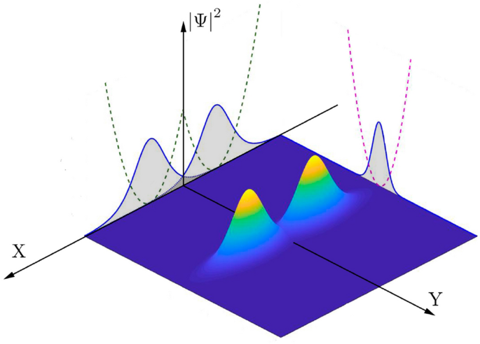
macroscopically populated modes as a result. QUANTIZATION OF COUPLED SOLITONS The sketch in Fig. 1 explains the two-soliton system described in our work. If trapping potential _V_(_x_) is

weak enough and the interaction among condensated particles is not so weak, the ansatz solution (3) is no longer suitable. For condensates with a negative scattering length, a bright soliton

solution is admitted for \(\Psi _{1,2}(x,t)\) in Eq. (2). In fact, in this case one can speak about two-soliton solution problem, which is well known in classical theory of solitons66. In

quantum theory, instead of Eq. (2), we deal with a bosonic field operator \({\hat{a}}(x,t)\propto {\hat{a}}_1+{\hat{a}}_2\), where \({\hat{a}}_{1,2}\equiv {\hat{a}}_{{1,2}}(x,t)\) are field

operators corresponding to mean-field amplitudes \(\Psi _{1,2}(x,t)\). We assume that experimental conditions allow the formation of atomic bright solitons in each of the wells. In

particular, these conditions may be realized by means of manipulation with weakly trapping potential _V_(_x_). Experimentally, this manipulation may be performed by a dipole trap and laser

field. Then, considering linear superposition state, one can write down the total Hamiltonian \({\hat{H}}\) for two BEC solitons in the second quantization form as $$\begin{aligned}

{\hat{H}} = \int _{-\infty }^\infty \sum _{j=1}^2\left( {\hat{a}}_j^\dag \left( -\frac{1}{2}\frac{\partial ^2}{\partial x^2}\right) {\hat{a}}_{j}dx\right) - \frac{u}{2}\int _{-\infty

}^\infty \Big ({\hat{a}}_1^\dag +{\hat{a}}_2^\dag \Big )^2\Big ({\hat{a}}_1+{\hat{a}}_2\Big )^2dx. \end{aligned}$$ (4) The annihilation (creation) operators of bosonic fields, denoted as

\({\hat{a}}_{j}\) (\({{\hat{a}}^\dag _{j}}\)) with \(j=1,2\), obey the commutation relations: $$\begin{aligned} {[}{\hat{a}}_i(x), {{\hat{a}}^\dag _{j}(x')}] = \delta

(x-x')\,\delta _{ij}; \quad i,j =1,2. \end{aligned}$$ (5) In the Hartree approximation for a large particle number, \(N>>1\), one can assume that the quantum _N_-particle

two-soliton state is the product of _N_ two-soliton states and can be written as67,68,69 $$\begin{aligned} \left| \Psi _N\right\rangle = \frac{1}{\sqrt{N!}}\left[ \int _{-\infty }^\infty

\left( \Psi _1(x,t){\hat{a}}_1^\dag e^{-i\beta _1t} + \Psi _2(x,t){\hat{a}}_2^\dag e^{-i\beta _2t}\right) dx\right] ^N\left| 0\right\rangle , \end{aligned}$$ (6) where \(\Psi _j(x,t)\) is

the unknown wave functions, and \(|0\rangle \equiv |0\rangle _1 |0\rangle _2\) denotes a two-mode vacuum state. The state given in Eq. (6) is normalized as \(\left\langle \Psi _N\big |\Psi

_N\right\rangle = 1\), and the bosonic field-operators \({\hat{a}}_{j}\) act on it as $$\begin{aligned} {\hat{a}}_j\left| \Psi _N\right\rangle = \sqrt{N}\Psi _j(x,t)e^{-i\beta _jt}\left|

\Psi _{N-1}\right\rangle . \end{aligned}$$ (7) Applying variational field theory approach based on the ansatz \(\Psi _j(x,t)\), one can obtain the Lagrangian density in the form:

$$\begin{aligned} L_0 = \frac{1}{2} \sum _{j=1}^2\left( i\left[ \Psi _j^*{\dot{\Psi }}_j - {\dot{\Psi }}_j^*\Psi _j\right] - \left| \frac{\partial \Psi _j}{\partial x}\right| ^2\right) +

\frac{uN}{2}\left( \Psi _1^*e^{i\beta _1t} +\Psi _2^*e^{i\beta _2t}\right) ^2\left( \Psi _1e^{-i\beta _1t}+\Psi _2e^{-i\beta _2t}\right) ^2, \end{aligned}$$ (8) where we suppose \(N-1\approx

N\) and omit common term _N_. Noteworthy, from Eq. (8), one can obtain the coupled GPEs for \(\Psi _j\)-functions as $$\begin{aligned} i\frac{\partial }{\partial t}\Psi _1= & {}

-\frac{1}{2}\frac{\partial ^2}{\partial x^2}\Psi _1 - uN\left( \left| \Psi _1\right| ^2 + 2\left| \Psi _2\right| ^2\right) \Psi _1\nonumber \\&- uN\left( \left| \Psi _2\right| ^2 +

2\left| \Psi _1\right| ^2\right) \Psi _2e^{-i\Omega t} - uN\Psi _1^*\Psi _2^2e^{-2i\Omega t} - uN\Psi _2^*\Psi _1^2e^{i\Omega t}, \end{aligned}$$ (9) $$\begin{aligned} i\frac{\partial

}{\partial t}\Psi _2= & {} -\frac{1}{2}\frac{\partial ^2}{\partial x^2}\Psi _2 - uN\left( \left| \Psi _2\right| ^2 + 2\left| \Psi _1\right| ^2\right) \Psi _2\nonumber \\&- uN\left(

\left| \Psi _1\right| ^2 + 2\left| \Psi _2\right| ^2\right) \Psi _1e^{i\Omega t} - uN\Psi _2^*\Psi _1^2e^{2i\Omega t} - uN\Psi _1^*\Psi _2^2e^{-i\Omega t}, \end{aligned}$$ (10) where

\(\Omega =\beta _2-\beta _1\) is the energy (frequency) spacing. The set of Eqs. (9) and (10) leads to the known problem for transitions between two lowest self-trapped states of condensates

in the nonlinear coupled mode approach if we account Eq. (3) for the representation of condensate wave functions \(\Psi _j(x,t)\)28,29. On the other hand, Eqs. (9) and (10) can be

recognized in the framework of soliton interaction problem that may be solved by means of perturbation theory for solitons66. In particular, in accordance with Karpman’s approach we can find

in Eq. (9) and (10) the terms proportional to \(\epsilon _{jk}=\Psi _j^*\Psi _k^2 + 2|\Psi _j|^2\Psi _k\), \(j,k=1,2\), \(j\ne k\), as perturbations for two fundamental bright soliton

solutions. Physically, \(\epsilon _{jk}\) implies the nonlinear Josephson coupling between the solitons. In this work we establish a variational approach for the solution of Eqs. (9) and

(10), cf.32. For the weakly coupled condensate states, i.e. for \(\epsilon _{jk}\simeq 0\), the set of Eqs. (9) and (10) can be reduced to two independent GPEs: $$\begin{aligned}

i\frac{\partial }{\partial t}\Psi _j = -\frac{1}{2}\frac{\partial ^2}{\partial x^2}\Psi _j - uN\left| \Psi _j\right| ^2\Psi _j, \end{aligned}$$ (11) which possess bright (non-moving) soliton

solutions $$\begin{aligned} {\Psi _j(x,t)} = \frac{N_j}{2}\sqrt{\frac{u}{N}}{{\,\text{ {sech}}\,}}\left[ \frac{uN_j}{2}x\right] e^{i\frac{u^2N_j^2}{8}t}. \end{aligned}$$ (12) In the case of

\(\epsilon _{jk}\ne 0\) and non-zero inter-soliton distance \(\delta\), we examine ansatzes for \(\Psi _j(x,t)\) in the form $$\begin{aligned} \Psi _1(x,t)= & {}

\frac{N_1}{2}\sqrt{\frac{u}{N}}{{\,\text{ {sech}}\,}}\left[ \frac{uN_1}{2}\left( x - \delta \right) \right] e^{i\theta _1}, \end{aligned}$$ (13) $$\begin{aligned} \Psi _2(x,t)= & {}

\frac{N_2}{2}\sqrt{\frac{u}{N}}{{\,\text{ {sech}}\,}}\left[ \frac{uN_2}{2}\left( x + \delta \right) \right] e^{i\theta _2}. \end{aligned}$$ (14) In particular, our approach presumes the

existence of two well distinguished solitons (separated by the small distance \(\delta\), with the shape preserved) interacting through dynamical variation of the particle numbers,

\(N_j\equiv N_j(t)\), and phases, \(\theta _j\equiv \theta _j(t)\), which occurs in the presence of weak coupling between the solitons. In other words, \(N_j\) and \(\theta _j\) should be

considered as time-dependent (variational) parameters. By substituting Eqs. (13) and (14) into (8) we obtain (up to the constant factor and term) $$\begin{aligned} L = \int _{-\infty

}^\infty L_0 dx\simeq - z{\dot{\theta }} + \Lambda z^2 + \frac{\Lambda }{2}\left( 1 - z^2\right) ^2I(z,\Delta )\left( \cos [2\Theta ]+2\right) + \Lambda \left( 1 - z^2\right) J(z,\Delta

)\cos [\Theta ], \end{aligned}$$ (15) where \(z=(N_2-N_1)/N\) (\(N_{1,2}=\frac{N}{2}(1\mp z)\)) is the particle number population imbalance; \(\Theta =\theta _2-\theta _1-(\beta _2-\beta

_1)t \equiv \theta - \Omega t\) is an effective time-dependent phase-shift between the solitons. Physically, \(\Omega\) is an angular frequency spacing between the ground and first excited

macroscopic states of the condensate; it represents a vital (measured) parameter for metrological purposes in this work. In Eq. (15), we also introduce the notation \(\Lambda =N^2u^2/16\)

and define the functionals $$\begin{aligned} I&\equiv I(z,\Delta ) = \int _{-\infty }^\infty {{\,\text{ {sech}}\,}}^2\left[ \left( 1 -z\right) \left( x-\Delta \right) \right] {{\,\text{

{sech}}\,}}^2\left[ \left( 1+z\right) \left( x+\Delta \right) \right] dx, \end{aligned}$$ (16) $$\begin{aligned} J&\equiv J(z,\Delta ) = \sum _{s=\pm 1}\left( \int _{-\infty }^\infty

\left( 1 +sz\right) ^2{{\,\text{ {sech}}\,}}^3\left[ \left( 1+sz\right) \left( x+s\Delta \right) \right] {{\,\text{ {sech}}\,}}\left[ \left( 1-sz\right) \left( x-s\Delta \right) \right]

\right) , \end{aligned}$$ (17) where \(\Delta \equiv ~\frac{Nu}{4}\delta\) is a normalized distance between solitons. Finally, by using Eq. (15) for the population imbalance and phase-shift

difference, _z_ and \(\Theta\), we obtain the set of equations $$\begin{aligned} {\dot{z}}= & {} \left( 1-z^2\right) \left\{ \left( 1-z^2\right) I\sin [2\Theta ] + J\sin [\Theta

]\right\} , \end{aligned}$$ (18) $$\begin{aligned} {\dot{\Theta }}= & {} - \frac{\Omega }{\Lambda } + 2z + \frac{{\text {d}}}{{\text {d}}z}\left\{ \frac{1}{2}\left( 1-z^2\right)

^2I\left( \cos [2\Theta ]+2\right) + \left( 1-z^2\right) J\cos [\Theta ]\right\} , \end{aligned}$$ (19) where dots denote the derivatives with respect to the renormalized time \(\tau

=\Lambda t\). In contrast to the problem with coupled Gaussian-shape condensates, the solutions of Eqs. (18) and (19) crucially depend on the features of governing functionals \(I(z,\Delta

)\) and \(J(z,\Delta )\), cf.28,29. In Supplementary Material we represent some analytical approximations for \(I(z,\Delta )\) and \(J(z,\Delta )\), in order to give a clear illustration.

STEADY-STATE (SS) SOLUTIONS STEADY-STATE SOLUTION FOR \(Z^2=1\) The steady-state (SS) solutions of Eqs. (18) and (19) play a crucial role for metrological purposes with coupled solitons47.

We start from the SS solution \(z^2=1\) of Eq. (18) by setting the time-derivatives to zero. As seen from Eqs. (16) and (17), in the limit of maximal population imbalance, \(z^2=1\), _I_ and

_J_ are independent on \(\Delta\) and approach $$\begin{aligned} I(z,\Delta )= & {} 1, \end{aligned}$$ (20) $$\begin{aligned} J(z,\Delta )= & {} \pi . \end{aligned}$$ (21)

Substituting \(z^2=1\) and Eqs. (20) and (21) into Eq. (19), we obtain $$\begin{aligned} z^2= & {} 1, \end{aligned}$$ (22) $$\begin{aligned} \Theta= & {} \arccos \left[

\frac{2\Lambda - {{\,\text{ {sign}}\,}}[z]\Omega }{2\pi \Lambda }\right]. \end{aligned}$$ (23) Notably, in the quantum domain the SS solutions shown in Eqs. (22) and (23) admit the existence

of quantum states with maximal population imbalance \(z = \pm 1\) and phase difference. The latter depends on the frequency spacing \(\Omega\), which is the object of precise measurement

with maximally path-entangled _N_00_N_-states in this paper. Below we perform the analysis of the SS solutions of Eqs. (18) and (19) in two limiting cases \(\Omega \ne 0\), \(\Delta \simeq

0\) and \(\Omega \simeq 0\), \(\Delta \ne 0\). SS SOLUTIONS FOR \(\THETA =0,\PI\) AND \(\DELTA \SIMEQ 0\) To find the SS solutions we rewrite Eq. (19) as $$\begin{aligned} \frac{\Omega

}{\Lambda } = 2z - 6z\left( 1-z^2\right) I + \frac{3}{2}\left( 1-z^2\right) ^2\frac{\partial I}{\partial z} - 2zJ + \left( 1-z^2\right) \frac{\partial J}{\partial z}, \end{aligned}$$ (24)

for \(\Theta =0\) and $$\begin{aligned} \frac{\Omega }{\Lambda } = 2z - 6z\left( 1-z^2\right) I + \frac{3}{2}\left( 1-z^2\right) ^2\frac{\partial I}{\partial z} + 2zJ - \left( 1-z^2\right)

\frac{\partial J}{\partial z}, \end{aligned}$$ (25) for \(\Theta =\pi\), respectively. In Supplementary Material we represent a polynomial approximation for _I_, _J_ functionals given in

Eqs. (16) and (17). Since the equations obtained from Eqs. (24) and (25) are quite cumbersome, here we just briefly analyze the results. In the limit of closely spaced solitons and \(\Theta

=0\), the population imbalance _z_ at equilibrium depends only on \(\Omega\) and obeys $$\begin{aligned} \frac{\Omega }{\Lambda } = 1.2 z^7 - 8 z^5 + 15 z^3 - 12.5 z. \end{aligned}$$ (26)

Similarly, for fixed soliton phase difference \(\Theta =\pi\) we have $$\begin{aligned} \frac{\Omega }{\Lambda } = 1.2 z^7 - 3.2 z^5 + 12.3 z^3 - 2 z. \end{aligned}$$ (27) We plot the

graphical solutions of Eqs. (26) and (27) in Fig. 2; the blue and red curves characterize the right parts of Eqs. (26) and (27), respectively. The straight lines in Fig. 2 correspond to

different values of the \(\Omega /\Lambda\) ratio. These lines cross the curves in the points indicating the solutions of Eqs. (26) and (27). Notice that the solid blue and red curves denote

the values of \(\Omega /\Lambda\) and _z_ corresponding to the stable SS solutions; while the dotted ones describe parametrically unstable solutions. As seen from Fig. 2, at phase

difference \(\Theta =0\) there exists one stable SS solution for any \(z\in [-0.7;0.7]\) and only unstable solutions for \(|z|>0.7\). At \(|\Omega /\Lambda |>1.55\pi\), no SS solutions

exist. On the other hand, at \(\Theta =\pi\) there exists a tiny region \(-0.1\pi \le \Omega /\Lambda \le 0.1\pi\) possessing two SS solutions simultaneously. One stable SS solution exists

within the domain \(0.1\pi <|\Omega /\Lambda |\le 2.64\pi\). SS SOLUTIONS FOR \(\THETA =0,\PI\) AND \(\OMEGA \SIMEQ 0\) At \(\Omega =0\) Eqs. (26) and (27) admit the SS solutions, which

look like: $$\begin{aligned}&z=0,\Theta =0, \end{aligned}$$ (28) $$\begin{aligned}&z=0,\Theta =\pi,\end{aligned}$$ (29) $$\begin{aligned}&z^2\approx 0.17, \Theta =\pi .

\end{aligned}$$ (30) As seen from Eq. (29), at relative phase \(\Theta =\pi\) Eq. (25) possesses three solutions: a parametrically unstable solution occurs at \(z=0\) and two degenerate SS

solutions appear for \(z=\pm z_0\). Here, \(z_0\) varies from 0.41 at \(\Delta \approx 0\) to 0.64 at \(\Delta \approx 2.8\) for non-zero soliton inter-distance, respectively. For \(\Delta

> 2.8\) these SS solutions do not exist. In Fig. 3 we represent a more general analysis of SS solutions for \(\Theta =0\) as functions of inter-soliton distance \(\Delta\) for different

\(\Omega\). For that we exploit the sixth-order polynomial approximation, see Supplementary Material. Notably, the dependence in Fig. 3 is similar to the one obtained with the

Lipkin–Meshkov–Glick (LMG) model, see e.g.70. The LMG model exhibits remarkable features including quantum phase transition and maximally entangled state formation, see e.g.71,72,73,74,75.

In our work, the distance between solitons plays a key role in this case. In particular, at \(\Omega \simeq 0\) there exists one solution at \(z=0\), stable at \(\Delta \le \Delta _c\approx

0.5867\). For \(\Delta >\Delta _c\) this solution becomes parametrically unstable. On the other hand, for \(\Delta >\Delta _c\) Eq. (24) possess the degenerate SS solutions similar to

the ones at \(\Theta =\pi\). The bifurcation for population imbalance _z_ occurs at \(\Delta =\Delta _c\); in Fig. 3 the \(z_+\) (upper,positive) and \(z_-\) (lower, negative) branches

characterize this bifurcation. In the vicinity of \(\Delta _c\) we can consider \(z_\pm =\pm z_0\), where $$\begin{aligned} z_0=1.2\sqrt{\Delta - \Delta _c}. \end{aligned}$$ (31) At \(\Omega

\ne 0\), the behavior of SS solutions become complicated with respect to the distance \(\Delta\)—see the green curves in Fig. 3. The solid curves correspond to SS solutions for different

\(\Delta\), while the dotted ones describe the unstable solutions. As clearly seen from Fig. 3, for \(\left| \Omega \right| >0\) there is no bifurcation for population imbalance _z_ and

two stationary solution branches \(z_{\pm }\) occur with \(|z_-|>|z_+|\). Notice, for \(\Omega >0\) there exists another critical point \(\Delta _c^{ub}>\Delta _c\), where the upper

branch \(z_+\) of SS solution appears. The numerical calculation for \(\Omega /\Lambda =0.05\pi\) in Fig. 3 gives \(\Delta _c^{ub}\approx 0.647\) or \(\Delta _- \approx 0.06\) in (35). For

these parameters \(z_+ \approx 0.2\) and \(z_- \approx -0.3\). On the other hand, at a relatively large values of parameter \(\Omega /\Lambda\), only one SS solution exists - see the red

curve in Fig. 3. MEAN-FIELD DYNAMICS SMALL AMPLITUDE OSCILLATIONS We start our analysis here from small amplitude oscillations close to SS solutions given in Eqs. (28)–(30). For that we

linearize Eqs. (18) and (19) in the vicinity of the solution in Eqs. (28) and (30), assuming \(0\le \Delta <0.6\) and \(\Omega {/\Lambda }<<1\). The first assumption allows us to

use the approximation of _I_, _J_-functionals by the fourth-degree polynomial, see Supplementary Material. For zero-phase oscillations, i.e. for \(\Theta \approx 0\) (\(\cos \left[ \Theta

\right] \approx 1\), \(\sin \left[ \Theta \right] \approx \Theta\)), from Eqs. (18) and (19) we obtain $$\begin{aligned} \ddot{z} + \omega _0^2(\Delta )z = f_0(\Delta )\frac{\Omega

}{{\Lambda }}, \end{aligned}$$ (32) with the solution $$\begin{aligned} z(\tau ) = A\cos \left[ \omega _0\tau \right] - \frac{\Omega }{{\Lambda }}\frac{f_0}{\omega _{0}^2}, \end{aligned}$$

(33) where _A_ and \(\omega _0(\Delta )=13.4\sqrt{0.37-\Delta ^2 - 0.25\Delta }\) are the amplitude and angular frequency of oscillations, respectively. Notice, here in (33) and thereafter

all frequencies \(\omega _j\) (\(j=0, \pi , ST\)) characterizing small amplitude oscillations are given in \(\Lambda ^{-1}\) units due to the time renormalization \(\tau = \Lambda t\)

performed earlier. The last term in Eq. (33) with \(f_0(\Delta )=5.36-0.8\Delta -4.22\Delta ^2\) plays a role of constant “external downward displacement force” that vanishes at \(\Omega

\simeq 0\). Notably, at \(\Delta >0.5\), the oscillations become anharmonic and \(z(\tau )\) diverges at \(\Delta >0.5867\). For \(\Delta =0\) the frequency of oscillations approaches

\(\omega _0 \approx 8.15\), that agrees with the numerical solution of Eqs. (18) and (19). At \(\Delta =\Delta _c\simeq 0.5867\) SS solution given in Eqs. (28) splits into two degenerate

solutions with \(z=\pm z_0\) and \(z_0\) determined by Eq. (31), see Fig. 3. Near these points the equation, similar to Eq. (32), has a form $$\begin{aligned} \ddot{z} + {\omega _{ST}^2}z =

- 18\Delta _-\sqrt{\Delta _-} - \frac{\Omega }{{\Lambda }}f(\Delta _-) \end{aligned}$$ (34) that implies a solution $$\begin{aligned} z(\tau ) = \pm \left( 1.2 - \frac{18\Delta _-}{{\omega

_{ST}^2}}\right) \sqrt{\Delta _-} + A\cos [{\omega _{ST}}\tau ] - \frac{\Omega }{{\Lambda }}\frac{f(\Delta _-)}{{\omega _{ST}^2}}, \end{aligned}$$ (35) where \(\Delta _-\equiv \Delta -\Delta

_c\), \({\omega _{ST}} = 14.53\sqrt{\Delta _{-} - 4.48\Delta _-^2 + 17.8\Delta _-^3 - 53.5\Delta _-^4}\) is the angular frequency of oscillations, and \(f = 3.4 - 7.26\Delta _- + 11\Delta

_-^2\) is the “external” force. A relative error for Eq. (35) is less than 5%. In the vicinity of SS points determined by Eq. (30), we obtain \(\pi\)-phase oscillations characterized by

$$\begin{aligned} z(\tau ) = \pm z_0 + A\cos \left[ \omega _{\pi }\tau \right] + \frac{\Omega }{{\Lambda }}\frac{f_{\pi }}{\omega _{\pi }^2}, \end{aligned}$$ (36) with \(\omega _{\pi } =

\sqrt{2-0.9\Delta ^2 - 0.3\Delta }\), \(f_{\pi } = 0.1\left( \Delta ^2 + 0.38\Delta + 5.5\right)\), and \(z_0\) determined in Eq. (30). For \(\Omega \simeq 0\) and \(\Delta =0\), the angular

frequency is \(\omega _{\pi } \approx 1.42\), which is much smaller than that in the zero-phase regime. The analysis of Eqs. (18) and (19) in the vicinity of Eq. (29) reveals that this

solution is parametrically unstable, and highly nonlinear behavior is expected. Indeed, a direct numerical simulation demonstrates anharmonic dynamics plotted in Fig. 4. For

\(0<|z|<0.5\) the nonlinear regime of self-trapping is observed,; while it turns into nonlinear oscillations at \(|z|>0.5\). The analysis of SS solution (22) and (23) reveals a

strong sensitivity to _z_-perturbation, when condition \(z^2=1\) is violated, the high-amplitude nonlinear oscillations occur. On the other hand, solution (22) and (23) is robust to

phase-perturbations, which is an important property for metrology. LARGE SEPARATION LIMIT, \(\DELTA>>1\) For a very large distance \(\Delta\) between the solitons, i.e.,

\(\Delta>>1\), the atom tunneling between them vanishes, and the solitons become independent. Strictly speaking, in the limit of \(\Delta \rightarrow \infty\) the functionals

\(I,J\rightarrow 0\), and Eqs.  (18) and (19) look like $$\begin{aligned} {\dot{z}}= & {} 0, \end{aligned}$$ (37) $$\begin{aligned} {\dot{\Theta }}= & {} - \frac{\Omega }{{\Lambda }}

+ 2z, \end{aligned}$$ (38) i.e., the population imbalance is a constant in time and the running-phase regime establishes. For large but finite \(\Delta\), SS solution having \(z=\pm z_0\)

with \(z_0\rightarrow 1\) exists for the zero-phase regime, \(\Theta =0\); for example, for \(\Delta =10\) the SS population imbalance is \(z_0\approx 0.96\). PHASE-SPACE ANALYSIS The

dynamical behavior of the coupled soliton system can be generalized in terms of a phase portrait of two dynamical variables _z_ and \(\Theta\), as shown in Figs. 5 and 6. In Fig. 5 we

represent \(z-\Theta\) phase-plane for \(\Omega =0\) and for different (increasing) values of distance \(\Delta\). We distinguish three different dynamic regimes. The solid curves correspond

to the oscillation regime when \(z(\tau )\) and \(\Theta (\tau )\) are some periodic functions of normalized time, see Eq. (33) and the red curve in Fig. 4. The dashed curves in Fig. 5

indicate the self-trapping regime when \(z(\tau )\) is periodic and the sign of _z_ does not change, see Eq. (36) and the blue curve in Fig. 4. Physically, this is the macroscopic quantum

self-trapping (MQST) regime characterized by a nonzero average population imbalance when the most of the particles are “trapped” within one of the solitons. At the same time, the behavior of

phase \(\Theta (\tau )\) may be quite complicated but periodic in time. On the other hand, for the running-phase regime depicted by the dashed-dotted curves, \(\Theta (\tau )\) grows

infinitely, see the green curve in Fig. 5b. Due to the symmetry that takes place at \(\Omega =0\), the running-phase can be achieved only with the MQST regime, see Fig. 5. As seen from Fig. 

5, the central area of nonlinear Rabi-like oscillations between the ground and first excited macroscopic states occur for a relatively small inter-soliton distance \(\Delta\) and are

inherent to zero-phase oscillations, see Fig. 5a. As discussed before, at \(\Delta =\Delta _c\approx 0.5867\) this area splits into two regions characterized by the MQST regimes, Fig. 5b.

This splitting occurs due to the bifurcation of population imbalance, see the black curve in Fig. 3. These regions are moving away from each other with growing \(\Delta\), see Fig. 5c–f.

Notably, the bifurcation effect and MQST states, which are the features of the coupled solitons (Fig. 1) at the zero-phase regime, do not occur for the condensates described by Gaussian

states28,29. The phase trajectories inherent to \(\pi\)-phase region \(\frac{\pi }{2}<\Theta <\frac{3\pi }{2}\) stay weakly perturbed until the second critical value \(\Delta \approx

2\), when the MQST regime in Fig. 5d changes to Rabi-like oscillations in Fig. 5e, then, approaches the running-phase at \(\Delta \approx 6\), see Fig. 5f. At large enough \(\Delta\), the

particle tunneling vanishes and the zero-phase MQST domains arise in the vicinity of population imbalance \(z=\pm 1\), Fig. 5f. The phase dynamics corresponds to the running-phase regime

with \(z = {{\,\text{ {const}}\,}}\), see Fig. 5f and Eqs.  (37) and (38). For non-zero \(\Omega\), the phase portrait becomes asymmetric, see Fig. 6. To elucidate the role of \(\Omega\), we

study the soliton interaction for a given inter-soliton distance \(\Delta =0.75>\Delta _c\) that corresponds to the one after the bifurcation. As seen from Fig. 6a, the phase portrait

does not change significantly for small \(\Omega {/\Lambda }\), cf. Fig. 5b. One of the SS solutions for zero and \(\pi\)-phase regimes disappears with increasing \(\Omega {/\Lambda }\);

then the running-phase regime establishes, see Fig. 6b. Further increasing of \(\Omega {/\Lambda }\) leads to vanishing the SS solution for zero-phase, Fig. 6c. Thus, phase portraits in

Figs. 5 and 6 demonstrate the existence of degenerate SSs for coupled solitons by varying \(\Delta\) and \(\Omega {/\Lambda }\). Such solutions, as we show below, may be exploited for the

macroscopic superposition soliton states formation in the quantum approach. QUANTUM METROLOGY WITH TWO-SOLITON STATES SOLITON SC-QUBIT STATES In this Section we demonstrate how two-soliton

quantum superposition states may be used for the parameter estimation and measurement procedure. In particular, we explore two degenerate states with population imbalance \(z=z_\pm\) for

these purposes. In the mean-field approximation \(z_\pm\) correspond to two SS solutions, which specify MQST regimes established in Fig. 5 for phases \(\Theta =0\) and \(\Theta =\pi\) (see

Eq. (30)), respectively. Strictly speaking, values \(z_\pm\) for \(\Theta =0\) are inherent to the upper and lower branches in Fig. 3 and appear above the critical distance \(\Delta _c\)

between the solitons, cf. Fig. 5b. In the quantum domain two degenerate SS solutions \(z_\pm\) (occurring simultaneously) determine the existence of macroscopic superposition states, which

correspond to SC- or _N_00_N_-states. Here, we specify necessary conditions for these states formation within the Hartree approach, cf.17,47. We generalize SC- and _N_00_N_-states as

macroscopic qubit states of the solitons, which we define as $$\begin{aligned} |\pi _0\rangle= & {} c_1|\Phi _1\rangle - c_2|\Phi _2\rangle , \end{aligned}$$ (39) $$\begin{aligned} |\pi

_1\rangle= & {} c_2|\Phi _1\rangle - c_1|\Phi _2\rangle , \end{aligned}$$ (40) where \(|\Phi _1\rangle\) and \(|\Phi _2\rangle\) are two macroscopic states representing two “halves” of

SC-, or _N_00_N_-states. Notice, operators \({\hat{\Pi }}_i= |\pi _i\rangle \langle \pi _i|\) realize a projection onto the superposition of states \(|\Phi _{1,2}\rangle\), which generally

are not orthogonal to each other obeying the condition $$\begin{aligned} \left\langle \Phi _1\Big |\Phi _2\right\rangle = \eta . \end{aligned}$$ (41) Simultaneously, we require the states in

Eqs. (39) and (40) to meet the normalization condition $$\begin{aligned} \left\langle \pi _i\Big |\pi _j\right\rangle = \delta _{ij},\quad i,j=0,1. \end{aligned}$$ (42) Now, we are able to

determine the coefficients \(c_{1,2}\), which fulfill Eqs. (41) and (42) and look like $$\begin{aligned} c_{1,2}=\sqrt{\frac{1\pm \sqrt{1-\eta ^2}}{2(1-\eta ^2)}}. \end{aligned}$$ (43) In

Eqs. (41) and (43), the parameter \(\eta\) defines the distinguishability of states \(|\Phi _{1,2}\rangle\). The case of \(\eta =1\) corresponds to completely indistinguishable states

\(|\Phi _{1,2}\rangle\). In this case one can assume that \(|\Phi _{1}\rangle\) and \(|\Phi _{2}\rangle\) represent the same state. On the other hand, the case of \(\eta =0\) (\(c_1=1\) and

\(c_2=0\)) characterizes completely orthogonal states \(|\Phi _{1,2}\rangle\); that becomes possible if \(|\Phi _{1,2}\rangle\) approach two-mode Fock states. In other words, this is a limit

of the _N_00_N_-state, for which the coupled solitons are examined. For \(\eta \ne 1\) it is instructive to represent soliton wave functions shown in Eqs. (13) and (14) in the form of

$$\begin{aligned} \Psi _1= & {} \frac{{\sqrt{uN}}}{4}(1-z){{\,\text{ {sech}}\,}}\left[ \left( 1-z\right) \left( \frac{uN}{4}x-\Delta \right) \right] e^{-i\frac{\theta }{2}},

\end{aligned}$$ (44) $$\begin{aligned} \Psi _2= & {} \frac{{\sqrt{uN}}}{4}(1+z){{\,\text{ {sech}}\,}}\left[ \left( 1+z\right) \left( \frac{uN}{4}x+\Delta \right) \right] e^{i\frac{\theta

}{2}}. \end{aligned}$$ (45) To be more specific, we examine here two soliton interaction with relative phase \(\Theta =0\) and intersoliton distances above critical values. From Eq. (6) we

obtain $$\begin{aligned} \left| \Phi _1\right\rangle= & {} \frac{1}{\sqrt{N!}}\left[ \int _{-\infty }^\infty \left( \Psi _1^{(+)}{\hat{a}}_1^\dag + \Psi _2^{(+)}{\hat{a}}_2^\dag \right)

dx \right] ^N\left| 0\right\rangle ,\end{aligned}$$ (46) $$\begin{aligned} \left| \Phi _2\right\rangle= & {} \frac{1}{\sqrt{N!}}\left[ \int _{-\infty }^\infty \left( \Psi

_1^{(-)}{\hat{a}}_1^\dag + \Psi _2^{(-)}{\hat{a}}_2^\dag \right) dx \right] ^N\left| 0\right\rangle , \end{aligned}$$ (47) for two “halves” of the SC-state, where $$\begin{aligned} \Psi

_1^{(\pm )}= & {} \frac{\sqrt{uN}}{4}(1-z_{\pm }){{\,\text{ {sech}}\,}}\left[ \left( 1-z_{\pm }\right) \left( \frac{uN}{4}x - \Delta \right) \right] , \end{aligned}$$ (48)

$$\begin{aligned} \Psi _2^{({\pm })}= & {} \frac{\sqrt{uN}}{4}(1+z_{\pm }){{\,\text{ {sech}}\,}}\left[ \left( 1+z_{\pm }\right) \left( \frac{uN}{4}x + \Delta \right) \right] .

\end{aligned}$$ (49) In Eqs. (48) and (49), \(z_{+}\) and \(z_{-}\) are two SS solutions corresponding to the upper and lower branches in Fig. 3, respectively. \(e^{-iN(\theta /2 + \beta

_1\tau )}\). In particular, for \(\Omega \approx 0\), we have \(z_{\pm }\rightarrow \pm z_0\). The scalar product for state given in Eqs. (46) and (47) is $$\begin{aligned} \eta = \left[

\int _{-\infty }^\infty \left( \Psi _1^{(+)}\Psi _1^{(-)} + \Psi _2^{(+)}\Psi _2^{(-)}\right) dx\right] ^N\equiv \varepsilon ^N, \end{aligned}$$ (50) where \(\varepsilon\) characterizes

solitons wave functions overlapping. Assuming non-zero and positive \(\Omega\) for \(\varepsilon\), one can obtain $$\begin{aligned} \varepsilon= & {} \frac{1}{2}\Bigg (\left(

1-\frac{z_++z_-}{2}\right) ^{{-1}} \left( 1-z_+\right) \left( 1-z_-\right) \left( 1-0.21\left[ \frac{z_+-z_-}{2-(z_+ + z_-)}\right] ^2\right) \nonumber \\&+\left(

1+\frac{z_++z_-}{2}\right) ^{{-1}}\left( 1+z_+\right) \left( 1+z_-\right) \left( 1-0.21\left[ \frac{z_+-z_-}{2+(z_++z_-)}\right] ^2\right) \Bigg ). \end{aligned}$$ (51) In Fig. 7, we

establish the principal features of coefficients shown in Eq. (43) and parameter \(\varepsilon\), see the inset in Fig. 7, as functions of \(\Delta\). The value of \(\Omega\) plays a

significant role in the distinguishability problem for states \(|\Phi _{1}\rangle\) and \(|\Phi _{2}\rangle\). In particular, for \(\Omega =0\) at the bifurcation point \(\Delta =\Delta

_c=0.5867\), we have \(\varepsilon =1\) that implies indistinguishable states \(|\Phi _{1}\rangle\) and \(|\Phi _{2}\rangle\), see the red curve in the inset of Fig. 7. In this limit, the

coefficients \(c_{1,2}\rightarrow \infty\). However, even for the small (positive) \(\Omega\), it follows from Eq. (51) that \(\varepsilon \ne 1\) for any \(\Delta >\Delta _c\), and

states \(|\Phi _{1}\rangle\), \(|\Phi _{2}\rangle\) are always distinguishable. In particular, it follows from zero-phase solution given in Eq. (35) that \(z_{\pm } = \pm \left( 1.2 -

\frac{18\Delta _-}{{\omega _{ST}^2}}\right) \sqrt{\Delta _-} - \frac{\Omega }{{\Lambda }}\frac{f(\Delta _-)}{{\omega _{ST}^2}}\) and \(|z_{+}|\ne |z_{-}|\). This is displayed by the green

curves in Fig. 7. The SS solutions possess \(c_1=1.057\), \(c_2=0.203\) for \(c_{1,2}\) that correspond to \(\Delta _c^{ub} \simeq 0.647\), \(\varepsilon \approx 0.9056\) for \(\Omega

{/\Lambda }=0.05\pi\). From Fig. 7, it is evident that coefficients \(c_{1,2}\) rapidly approach (due to the factor _N_) levels \(c_{1}=1\), \(c_{2}=0\) (completely distinguishable

macroscopic SC soliton states), when \(\Delta\) increases. In this limit, as seen from Fig. 3, \(z_{\pm }\) approaches \(\pm z_0\), and from Eq. (51) we obtain $$\begin{aligned} \varepsilon

\approx (1-z_0^2)(1-0.21z_0^2). \end{aligned}$$ (52) Practically, in this limit the red and green curves coincide in Fig. 7. Remarkably, the case of \(\eta =0\) characterizes completely

orthogonal states \(|\Phi _{1,2}\rangle\) in (41) and (50); that becomes possible if \(|\Phi _{1,2}\rangle\) approach two-mode Fock states. In other words, this is a limit of the

_N_00_N_-state, for which we examine the coupled solitons. In this limit, the relative soliton phase approaches (23). PARAMETER ESTIMATION WITH MACROSCOPIC QUBIT STATES We can exploit states

shown in Eqs. (46) and (47) in metrological measurement for arbitrary phase \(\phi _N\) estimation. In general, suppose that two-soliton quantum system is prepared in state \(|\psi

\rangle\), which carries information about some parameter \(\Gamma\) that we would like to estimate. In this work we are interested in fundamental bound for a positive operator valued

measurement (POVM) and consider pure states of the quantum system. The precision of the estimation of some parameter \(\Gamma\) is described by the error propagation formula27 given as

$$\begin{aligned} \sigma _\Gamma = \frac{\sqrt{\left\langle \psi |(\Delta {\hat{\Pi }} )^2|\psi \right\rangle }}{\left| \frac{\partial \left\langle \psi | {\hat{\Pi }}|\psi \right\rangle

}{\partial \Gamma }\right| }, \end{aligned}$$ (53) where within the quantum metrology approach \(\left\langle \psi |(\Delta {\hat{\Pi }})^2|\psi \right\rangle = {\left\langle \psi |{\hat{\Pi

}}^2 |\psi \right\rangle - \left\langle \psi |{\hat{\Pi }}|\psi \right\rangle }^2\) represents the variance of fluctuations of some operator \({\hat{\Pi }}\) that corresponds to the

measurement procedure performed with the (pure) state \(|\psi \rangle\). Typically, such procedures are based on appropriate interferometric schemes and use quantum superpositions initially

prepared and then explored for measurement and estimation of parameter \(\Gamma\), cf.76. In other words, the measurement procedure, that we consider here, includes three important steps

involving two-soliton state preparation, subsequent phase \(\phi _N\) accumulation and measurement (estimation), cf.9. Practically, two-soliton state preparation involves a splitting

procedure, which corresponds to the first beam splitter action in traditional Mach–Zehnder interferometer, see e.g.10. At this stage we suppose \(\Omega\) vanishing. Then, we assume that the

output state \(|\psi \rangle\) of quantum system that we use for measurement and parameter (phase) estimation is represented as $$\begin{aligned} |\psi \rangle =\frac{1}{\sqrt{2}}(|\pi

_0\rangle {-}e^{i\phi _N}|\pi _1\rangle ), \end{aligned}$$ (54) where \(\phi _N\) is a relative (estimated) phase between states \(|\pi _0\rangle\) and \(|\pi _1\rangle\), defined as

$$\begin{aligned} \phi _N=N\Theta _{\Omega }+N\varphi . \end{aligned}$$ (55) In (55) \(\Theta _{\Omega }\) is the phase occurring between the solitons within the time \(\tau _{\Omega }\) for

non-vanishing \(\Omega\); \(\varphi =\omega \tau _{\omega }\equiv \Gamma\) is an additional phase accumulated during time \(\tau _{\omega }\). Thus, we suppose that the measurement and

parameter-estimation procedure generally includes two stages characterized by total phase \(\phi _N\). At first, let us examine the problem of estimation some arbitrary phase \(\varphi\),

which may be created after two-soliton state formation. The role of soliton phase difference \(\Theta _{\Omega }\) is negligible here, if we consider soliton interaction regimes with

vanishing \(\Omega\) (or very short time interval \(\tau _{\Omega }\)), proposing \(\Theta =0\), or \(\Theta =\pi\). In this limit we exploit soliton SC-state to estimate phase parameter

\(\phi _N\simeq N\varphi\). We assume in (54) that phase \(\phi _N\simeq N\Gamma\) contains all the information about measured parameter \(\Gamma\) and linearly depends on particle number

_N_. Notice, this assumption is valid only in the linear metrology approach framework, cf.30. Then, we define a complete set of operators \({\hat{\Sigma }}_j\), \(j=1,2,3\) (cf.60)

$$\begin{aligned} {\hat{\Sigma }}_0= & {} \left| \pi _1\right\rangle \left\langle \pi _1\right| + \left| \pi _0\right\rangle \left\langle \pi _0\right| , \end{aligned}$$ (56)

$$\begin{aligned} {\hat{\Sigma }}_1= & {} \left| \pi _1\right\rangle \left\langle \pi _1\right| - \left| \pi _0\right\rangle \left\langle \pi _0\right| , \end{aligned}$$ (57)

$$\begin{aligned} {\hat{\Sigma }}_2= & {} \left| \pi _0\right\rangle \left\langle \pi _1\right| + \left| \pi _1\right\rangle \left\langle \pi _0\right| , \end{aligned}$$ (58)

$$\begin{aligned} {\hat{\Sigma }}_3= & {} i( \left| \pi _0\right\rangle \left\langle \pi _1\right| - \left| \pi _1\right\rangle \left\langle \pi _0\right| ), \end{aligned}$$ (59) which

obey the SU(2) algebra commutation relation. The meaning of sigma-operators is evident from their definitions given in Eqs. (56)–(59). Physically, operators (56)–(59) are similar to the

Stokes parameters, which characterize polarization qubit (two-mode) state, cf.77 . Due to the properties shown in Eq. (42), the states \(|\pi _{i}\rangle\) are suitable candidates for the

macroscopic qubit states, which we can define by mapping \(|\pi _{0}\rangle \rightarrow |{\mathbf {0}}\rangle\) and \(|\pi _{1}\rangle \rightarrow |{\mathbf {1}}\rangle\), respectively53,78.

In this form we can use them for POVM measurements defined with operators79 $$\begin{aligned} E_1\equiv & {} \frac{\sqrt{2}}{1+\sqrt{2}}|{\mathbf {1}}\rangle \left\langle {\mathbf {1}}

\right| =\frac{1}{\sqrt{2}(1+\sqrt{2})}({\hat{\Sigma }}_0+{\hat{\Sigma }}_1), \end{aligned}$$ (60) $$\begin{aligned} E_2\equiv & {} \frac{1}{\sqrt{2}(1+\sqrt{2})}(|{\mathbf {0}}\rangle

-|{\mathbf {1}}\rangle )(\langle {\mathbf {0}}| + \langle {\mathbf {1}}|) =-\frac{1}{\sqrt{2}(1+\sqrt{2})}({\hat{\Sigma }}_1+i{\hat{\Sigma }}_3), \end{aligned}$$ (61) $$\begin{aligned}

E_3\equiv & {} I-E_1-E_2. \end{aligned}$$ (62) Importantly, current quantum technologies permit POVM tomography54.In particular, POVM tomography involves reconstruction of the Stokes

vector for the polarization qubit and requires four measurements at least, cf.80. In Ref.81 we suggested a special multiport interferometer for simultaneous measurement of all the Stokes

parameters, which are relevant to macroscopic two-mode quantum state characterization. The proposed interferometer consists of a set of beam splitters and simple phase-shift device, which

may be implemented in the atomic optics domain by relevant procedures performed with two-mode (spinor) atomic condensates, cf.9,10. Average values of sigma-operators in Eqs. (56)–(59) can be

obtained with the help of Eqs. (42) and (54), resulting in $$\begin{aligned} \left\langle {\hat{\Sigma }}_1\right\rangle= & {} 0, \end{aligned}$$ (63) $$\begin{aligned} \left\langle

{\hat{\Sigma }}_2\right\rangle= & {} \cos [\phi _N],\end{aligned}$$ (64) $$\begin{aligned} \left\langle {\hat{\Sigma }}_3\right\rangle= & {} \sin [\phi _N]. \end{aligned}$$ (65) From

Eqs. (63)–(65) it follows that only \(\left\langle {\hat{\Sigma }}_{2,3}\right\rangle\) contain the information about the desired phase \(\phi _N\). To estimate the sensitivity of phase

measurement, we can assume here \(\phi _N=N\Gamma\) and use Eq. (53) with the measured operator \({\hat{\Pi }}\equiv \hat{\Sigma _2}\). Taking into account \(\left\langle {\hat{\Sigma

}}_2^2\right\rangle = 1\) for the variance of fluctuations \(\left\langle (\Delta {\hat{\Sigma }}_2)^2\right\rangle\), we obtain $$\begin{aligned} \left\langle (\Delta {\hat{\Sigma

}}_2)^2\right\rangle = \sin ^2[N\Gamma ]. \end{aligned}$$ (66) Finally, from Eqs. (53) and (66) for the phase error propagation we get $$\begin{aligned} \sigma _\Gamma = \frac{1}{N},

\end{aligned}$$ (47) that clearly corresponds to the HL of arbitrary (linearly _N_-dependent) phase estimation and explores the sigma-operator measurement procedure. NONLINEAR METROLOGY

APPROACH FOR FREQUENCY MEASUREMENT, \(\GAMMA \EQUIV \OMEGA\) Now, we represent another particularly important case which relates to angular frequency \(\Omega\) measurement that

characterizes energy spacing between the ground and first excited macroscopic states. In particular, we suppose that all the information about \(\Omega\) is embodied in phase \(\phi

_N=N\Theta _{\Omega }\); the measurement and estimation procedure is realized immediately after period \(\tau _{\Omega }\). In other words, here we ignore linear (in respect of particle

number _N_, frequency \(\omega\) and time duration \(\tau _{\omega }\)) phase shift \(\varphi\), cf. (55). The SS solutions given in (22) and (23), which correspond to the maximal population

imbalance, \(z^2=1\), allow us to prepare the maximally path-entangled superposition state, a.k.a. _N_00_N_-state. As seen from Eq. (23), the solution with \(z=1\) exists when \(-2(\pi

-1)\le \Omega /\Lambda \le 2(\pi +1)\). Similarly, the domain of solution \(z=-1\) is \(-2(\pi +1)\le \Omega /\Lambda \le 2(\pi -1)\). To achieve the superposition _N_00_N_-state formation,

we require both solutions to exist simultaneously. This restricts the domain of \(\Omega\) as \(-2(\pi -1)\le \Omega /\Lambda \le 2(\pi -1)\). Substituting \(z =\pm 1\) into Eqs. (44) and

(45) we obtain $$\begin{aligned} \Psi _1= & {} \frac{\sqrt{uN}}{2}{{\,\text{ {sech}}\,}}\left[ \left( \frac{uN}{2}x-2\Delta \right) \right] e^{-i\frac{\theta }{2}}, \end{aligned}$$ (68)

$$\begin{aligned} \Psi _2= & {} \frac{\sqrt{uN}}{2}{{\,\text{ {sech}}\,}}\left[ \left( \frac{uN}{2}x+2\Delta \right) \right] e^{i\frac{\theta }{2}}, \end{aligned}$$ (69) which are

relevant to the _N_00_N_-state’s two “halves” defined as $$\begin{aligned} \left| N0\right\rangle= & {} \frac{1}{\sqrt{N!}}\left[ \int _{-\infty }^\infty \Psi _1{\hat{a}}_1^\dag

dx\right] ^N\left| 0\right\rangle, \end{aligned}$$ (70) $$\begin{aligned} \left| 0N\right\rangle= & {} \frac{1}{\sqrt{N!}}\left[ \int _{-\infty }^\infty \Psi _2{\hat{a}}_2^\dag dx\right]

^N\left| 0\right\rangle . \end{aligned}$$ (71) Considering the superposition of states shown in Eqs. (70) and (71) and omitting unimportant common phase \(e^{iN\left( 0.5\theta ^{(-)}-\beta

_1t\right) }\), from (54) we arrive at $$\begin{aligned} {|\psi \rangle \equiv }\left| N00N\right\rangle = \frac{1}{\sqrt{2}} \left( \left| N0\right\rangle + e^{iN{\Theta _{\Omega }}}\left|

0N\right\rangle \right) , \end{aligned}$$ (72) that represents the _N_00_N_-state of coupled BEC solitons for our problem. Here, $$\begin{aligned} {\Theta _{\Omega }} = \frac{\Theta ^{(+)}

+ \Theta ^{(-)}}{2} = \frac{1}{2}\left( \arccos \left[ \frac{2\Lambda - \Omega }{2\pi \Lambda }\right] + \arccos \left[ \frac{2\Lambda + \Omega }{2\pi \Lambda }\right] \right) ,

\end{aligned}$$ (73) is the phase shift that contains the \(\Omega\)-parameter required for estimation. Remarkably, we deal here with the nonlinear metrology approach since two-soliton phase

\(\Theta _{\Omega }\) nonlinearly depends on \(\Omega\) and parameter \(\Lambda\) (particle number _N_), cf.31,32,47. To study the ultimate achievable precision of such a measurement with

state (72), we consider the quantum Cramer–Rao bound9 $$\begin{aligned} \sigma _\Omega = \frac{1}{\sqrt{\nu F_Q}}, \end{aligned}$$ (74) where \(\nu\) is the number of subsequent measurements

(for the sake of simplicity we take \(\nu =1\)) and \(F_Q\) is the quantum Fisher information. The latter is defined for the pure state \(\left| \psi \right\rangle\) of the system as

$$\begin{aligned} F_Q = 4\left[ \left\langle \psi '_\Omega |\psi '_\Omega \right\rangle - \left| \left\langle \psi |\psi '_\Omega \right\rangle \right| ^2\right] ,

\end{aligned}$$ (75) where \(\left| \psi '_\Omega \right\rangle \equiv \partial \left| \psi \right\rangle /\partial \Omega\). Substituting (72) with \(|\psi \rangle \equiv

|N00N\rangle\) into (75) and then into (74) we get $$\begin{aligned} \sigma _\Omega = \frac{1}{N}\left| \frac{\partial {\Theta _{\Omega }}}{\partial \Omega }\right| ^{-1}. \end{aligned}$$

(76) Notice, Eq. (76) directly results from (53) with (72) and (73). Comparing Eq. (72) with Eq. (54), we can conclude that the _N_00_N_-state “halves” \(\left| N0\right\rangle\) and

\(\left| 0N\right\rangle\) in Eq. (72) may be associated with states \(|\pi _0\rangle\) and \(|\pi _1\rangle\), respectively. To estimate the sensitivity of the \(\Omega\)-measurement, we

use Eq. (76) with measured operator \({\hat{\Pi }}\equiv {\hat{\Sigma }}\) defined as $$\begin{aligned} {\hat{\Sigma }} = \left| N0\right\rangle \left\langle 0N\right| + \left|

0N\right\rangle \left\langle N0\right|. \end{aligned}$$ (77) Since states shown in Eq. (77) are orthogonal, the mean value of Eq. (77) is $$\begin{aligned} \left\langle {\hat{\Sigma

}}\right\rangle = \cos [N\Theta _{{\Omega }}]. \end{aligned}$$ (78) Figure 8a demonstrates \(\left\langle {\hat{\Sigma }}\right\rangle\) as a function of \(\Omega /\Lambda\). Notice, the

interference pattern in Fig. 8a exhibits an essentially nonlinear behavior for measured \(\left\langle {\hat{\Sigma }}\right\rangle\). The variance of fluctuations \(\left\langle (\Delta

{\hat{\Sigma }})^2\right\rangle\) for the measured sigma-operator reads as $$\begin{aligned} \left\langle (\Delta {\hat{\Sigma }})^2\right\rangle = \sin ^2[N\Theta _{{\Omega }}].

\end{aligned}$$ (79) Now, by using Eqs. (73) and (76) we can easily find the propagation error for the \(\Omega\)-estimation as $$\begin{aligned} \sigma _\Omega = \frac{2\Lambda }{N}\left|

\frac{\sqrt{4\pi ^2 -(2+\Omega /\Lambda )^2}\sqrt{4\pi ^2-(2-\Omega /\Lambda )^2}}{\sqrt{4\pi ^2-(2+\Omega /\Lambda )^2} - \sqrt{4\pi ^2-(2-\Omega /\Lambda )^2}}\right| . \end{aligned}$$

(80) Then, we choose the optimal estimation area for \(\Omega\), with the best sensitivity reached, in the vicinity of the domain border at \(\Omega /\Lambda \rightarrow 2(\pi -1)\). In this

limit, Eq. (80) approaches $$\begin{aligned} \sigma _\Omega \simeq \frac{10\Lambda }{N}\frac{1.17\sqrt{2(\pi -1) - \Omega /\Lambda }}{1.65 - \sqrt{2(\pi -1) - \Omega /\Lambda }}.

\end{aligned}$$ (81) Equations (80) and (81) demonstrate one of the important results of this paper: for a given \(\Lambda\), that characterizes atomic condensate peculiarities, Eq. (81)

demonstrates Heisenberg scaling for frequency measurement sensitivity. At the same, time (80) and (81) exhibit some specific peculiarities in two limiting cases, which are inherent to the

highly nonlinear interference pattern represented in Fig. 8a. First, (80) is non-applicable (\(\sigma _\Omega \rightarrow \infty\) ) for \(\Omega =0\) since \({\left| \frac{\partial \

\left\langle {\hat{\Sigma }}\right\rangle }{\partial \Omega }\right| =0}\). Second, \(\sigma _\Omega \rightarrow 0\) if \(\Omega /\Lambda \rightarrow 2(\pi -1)\). Qualitatively this

situation is shown in Fig. 8b. Geometrically \(\tan [\alpha ]={\left| \frac{\partial \ \left\langle {\hat{\Sigma }}\right\rangle }{\partial \Omega }\right| }\) determines the slope of the

tangent to the curve characterizing the interference pattern, cf.27. The blue curve in Fig. 8b corresponds to the ideal interference pattern shown in Fig. 8a. Obviously, the tangent is

parallel to the abscissa axis in \(\Omega =0\) point. At the border of the pattern the tangent tends to be perpendicular to the \(\Omega\) axis and \(\sigma _\Omega \rightarrow 0\).

Physically, such a behavior is not surprising and corresponds to the essentially nonlinear (in respect of \(\Omega\) ) metrology limit that establishes the interference pattern in Fig. 8a.

In this case one can obtain the SH scaling for the phase parameter measurement and estimation, cf.30,32,33,34. EXPERIMENTAL FEASIBILITY OF QUANTUM METROLOGY WITH CONDENSATE BRIGHT SOLITONS

Let us briefly discuss the feasibility of experimental observation of the proposed high-precision measurements with mesoscopic superposition states in the presence of losses for the quantum

soliton system in Fig. 1. A purely quantum theory (beyond the Hartree approach) of coupled solitons established in Fig. 1 represents a non-trivial task due to the essentially nonlinear

character of particle tunneling between the solitons. However, the results for quantum solitons obtained in48 allow to present here some simple arguments on the feasibility of

quantum-enhanced metrology effects observation with coupled solitons discussed above. First, we examine the influence of particle losses on _N_00_N_-state (72). The losses that occur between

the two-soliton quantum state preparation and the measurement are similar to the action of some fictitious beam splitters, which introduce additional noises36,48. As shown in48, the

resulting quantum state of coupled (in the transverse plane) solitons may be characterized by the superposition of the Fock states with highly populated _N_00_N_-components. In the presence

of few (even one) particle losses such a state experiences a partial collapse with the formation of the highly asymmetric _N_00_N_-like state. We represent here such a state as

$$\begin{aligned} \left| N00N\right\rangle _{\gamma } = \frac{1}{\sqrt{1+\gamma ^2}}\left( \gamma \left| N0\right\rangle + e^{iN\Theta _{\Omega }}\left| 0N\right\rangle \right) ,

\end{aligned}$$ (82) where \(\gamma\) is a vanishing parameter characterizing the _N_00_N_-state decay in the presence of losses. \(\gamma\) may be estimated as \(\gamma \simeq 0.25

N^{-1/2}\) if one particle is lost from the coupled solitons, see for details48. Now, instead of (78) we obtain $$\begin{aligned} \left\langle {\hat{\Sigma }}\right\rangle \equiv

\left\langle {\hat{\Sigma }} \right\rangle _\gamma = \frac{2\gamma }{1+\gamma ^2}\cos [N\Theta _{{\Omega }}]. \end{aligned}$$ (83) Equation (83) manifests a vanishing interference pattern in

the limit of \(\gamma \rightarrow 0\). Equations (78) and (83) allow to establish relations between angles \(\alpha\) and \(\alpha _\gamma\): $$\begin{aligned} \tan [\alpha _\gamma ]

=\frac{2\gamma }{1+\gamma ^2}\tan [\alpha ]\simeq \frac{1}{2\sqrt{N}}\tan [\alpha ]. \end{aligned}$$ (84) The last relation in (84) is valid for a single particle loss. Equation (84)

possesses a simple geometric interpretation: the particle losses reduce the slope of the tangent to the curve more than \(\sqrt{N}\) times. Moreover, from definition Eqs. (53) and (82) it is

possible to show that the propagation error for the \(\Omega\)-estimation in the presence of losses that we define as \(\sigma _{\Omega ,\gamma }\) also increases in \(2\sqrt{N}\) times in

comparison with \(\sigma _{\Omega }\) established in (80). The red curve in Fig. 8b qualitatively demonstrates how losses case the decrease of the \(\alpha\) angle and increase of \(\sigma

_\Omega\). Thus, losses lead to the decoherence of an interference pattern, cf.82, and, as a result, the slope of the curve modifies. Hence, in the real-world \(\Omega\) measurement, for

essential amount of losses the accuracy \(\sigma _{\Omega ,\gamma }\propto 1/\sqrt{N}\) corresponds to the standard quantum limit of frequency estimation. It is worth to notice that qubit

states  (39) and (40) based on SC-state solutions for \(|\Phi _1\rangle\) and \(|\Phi _2\rangle\) “halves” should be more robust to small particle losses since each “halve” posses a binomial

distribution of mesoscopic (or macroscopic) number of particles, see (46) and (47). Now let us discuss which type of losses are actual for two-soliton states and how we can avoid them

obtaining quantum-enhanced metrology discussed above. Previously, in Ref.48, and then in Ref.84 we examined this problem for quantum solitons possessing simple Josephson coupling in another,

transverse, configuration of soliton interaction, which is reminiscent to commonly considered weakly-coupled condensates possessing Gaussian wave functions, cf.12,13,14,16. From the

experimental point of view, recent BEC soliton experiments with lithium condensates demonstrated that one- and three-body losses may be recognized as major detrimental effects for quantum

solitons, cf.48,85,86. In particular, we examine here time scale \(\tau _d\), in which an one-particle-loss event takes place in average; \(\tau _d\) may be calculated as (cf.85,86)

$$\begin{aligned} \tau _d = \left( \frac{N}{\tau _1} + \frac{N^5}{3\tau _3}\right) ^{-1}, \end{aligned}$$ (85) where \(\tau _1\equiv 1/K_1\) and \(\tau _3\) are characteristic times for one-

and three-body losses, respectively. The temporal parameters introduced in (85) are dimensionless (we normalized time variable on characteristic time scale \(1/\omega _{\perp }\), as it is

established in (1)). Notice, apart from our approach represented in Ref.48, authors in Refs.85,86 take into account the density heterogeneity within soliton spatial distribution, which

implies the fifth order power in respect of particle number _N_ in Eq. (85) for three-body recombination losses. We can represent \(\tau _3\) in terms of dimensionless nonlinear strength _u_

as $$\begin{aligned} \tau _3 = \frac{90\pi ^2}{u^2K_3}\equiv \frac{5.625\pi ^2 N^2}{\Lambda K_3}, \end{aligned}$$ (86) where \(K_3\) is a constant (normalized on \(\omega _\perp a_{\perp

}^6\)) responsible for three-body recombination losses. Another important characteristic time is $$\begin{aligned} \tau _{sol} = \frac{1}{u^2N^2}\equiv \frac{1}{16\Lambda }, \end{aligned}$$

(87) which results from the energy-time uncertainty relation. We consider particle losses as adiabatic processes occurring slowly in comparison with \(\tau _{sol}\), cf.15,85,86. Thus, we

can impose that the changes in particle number _N_ (loss events) should take place on time scales sufficiently longer than characteristic time scales \(\tau _{sol}, \tau _{\Omega }, \tau

_{\omega }\). Strictly speaking, we require $$\begin{aligned} \tau _{sol}< \tau _{\Omega }, \tau _{\omega } < \tau _{d}, \end{aligned}$$ (88) as a necessary condition for observation

of the proposed measurement and estimation approach with solitons. For numerical estimations we use here experimentally accessible parameters of bright solitons observed with lithium BEC42.

A harmonic magneto-optical potential was exploited to trap the BEC of \({}^7\)Li atoms with characteristic frequency \(\omega _\perp = 2\pi \times 710\) Hz, providing characteristic spatial

scale \(a_\perp =1.4\times 10^{-6}\) m. The condensate soliton was formed at s-wave scattering length \(a_{sc}=-0.21\times 10^{-9}\) m manipulated via the Feshbach resonance technique.

Coefficients \(K_1\) and \(K_3\) for one- and three-body losses may be estimated (in physical units) as \(K_1=0.05\,\hbox {s}{}^{-1}\) and \(K_3=6\times 10^{-42}\,\hbox {m}^6\hbox

{s}^{-1}\), respectively, cf.86. Finally, for mesoscopic particle number \(N\simeq 1000\) from (85) we obtain estimation characteristic time scales as \(\tau _d = 87.4\), \(\tau _{sol} =

0.28\) (\(\Lambda \approx 0.22\)), which imply \(\tau _d \simeq 19.6\) ms and \(\tau _{sol} = 63\) \(\mu\)s given in physical units, respectively. It is worth noticing that three-body losses

are quite small in this limit and may be neglected, cf.48. Our estimations show that the last term in (85) relevant to three-body losses becomes compatible with the first one for particle

number \(N\simeq 3000\). Obviously, three-body losses dominate with increasing particle number _N_, cf.86. However, bright solitons occurring in the condensates with a negative scattering

length possess a wave-function collapse for macroscopically large _N_42. Roughly speaking, condensate bright solitons collapse if the number of atoms exceeds the critical value, \(N_c=0.67

a_{\perp }/|a_{sc}|\)39, which implies \(uN_c\approx 4.2\) (in Ref.42 authors demonstrated that \(N_c\) is relevant to the number of atoms \(5.2\times 10^3\)). In Refs.48,84 we proposed

coupled bright solitons for quantum metrology purposes containing few hundreds of condensate particles. Thus, our approach for the measurement and parameter estimation procedure requires

time scales shorter than \(\tau _d\) and a moderate (mesoscopic) number of condensate particles, see (88). Notice, that in Ref.42 the observation time was less than 10 ms. Quantum properties

of solitons applied to metrology will become possible with further improvements (in respect of particle number) of current experiments with BEC solitons43 and cf.84. In the real-world

experiment, on-chip Mach–Zehnder interferometer technology for atomic condensates may be useful for the frequency parameter \(\Omega\) estimation described above, cf.10. In particular, an

accumulated (additional) phase \(\varphi\) can also help select a measurement window in respect to parameter \(\Omega\) for the interference pattern given in Fig. 8a. The magnetic field can

be implemented for \(\Omega\) tuning and manipulation. At the same time, magnetic field may be used to tune and enhance atom-atom scattering length11. Furthermore, the accuracy at Heisenberg

scaling and beyond for parameter (phase) estimation alternatively may be obtained by the parity measurement procedure instead of \({\hat{\Sigma }}\)-operator exploring, see47,60 and,

especially, Ref.83 for recent progress achieved with the parity-based detection technique for atomic quantum states. Thus, we expect the on-chip Mach–Zehnder interferometer containing

soliton Josephson junctions to be in focus of experimental research in the near future. CONCLUSION In summary, we have considered the problem of two-soliton formation for 1D BECs trapped

effectively in a double-well potential. The analytical solutions of these soliton Josephson junctions and corresponding phase portraits exhibit the occurrence of novel macroscopic quantum

selft-trapping (MQST) phases in contrast to the condensates with only Gaussian wave functions. With these soliton states, we have also explored the formation of the Schrödinger-cat (SC)

state in the framework of the Hartree approximation. In particular, we have analyzed the distinguishability problem for binary (non-orthogonal) macroscopic states. Compared to the known

results47, finite frequency spacing \(\Omega\) leads to distinguishable macroscopic states for condensate solitons. This circumstance may be important for the experimental design of the

SC-states. The important part of this work is devoted to the applicability of predicted states for quantum metrology. In the framework of the linear metrology approach, by utilizing the

macroscopic qubits problem with the interacting BEC solitons, one can apply the sigma-operators to elucidate the measurement and subsequent estimation of an arbitrary phase, that linearly

depends on the particle number, up to the HL. Notably, the sigma-operators relate to the POVM detection tomography, which is similar to the Stokes parameters measurement within the qubit

state reconstruction procedure. On the other hand, the phase estimation procedure for the phase-dependent sigma-operator can be realized by means of the parity measurement technique that

produces the same accuracy for phase estimation. We have shown that in the limit of soliton state solution with the population imbalance \(|z|=\pm 1\) the coupled soliton system admits the

maximally path-entangled _N_00_N_-state formation. In the framework of the nonlinear metrology approach, we have also demonstrated the possibility to estimate frequency \(\Omega\) at the HL

and beyond by soliton phase difference estimation. The SH scaling for frequency estimation becomes possible due to the nonlinear interference pattern, which occurs for the relative soliton

phase. The numerical estimation for characteristic time scales of one- and three-body losses which are based on the existing experimental results with condensate bright solitons,

demonstrates the feasibility of the experimental realization of the proposed quantum metrological schemes possessing moderate losses in the nearest future. At the same time, it is

instructive to analyze quantum regimes with coupled solitons (see Fig. 1) established in this work. We plan a more detailed study of the quantum phase transition problem that is inherent to

the LMG model and has not been verified in the paper. We will publish the analysis of these problems in the future. REFERENCES * Udem, T., Holzwarth, R. & Hänsch, T. W. Optical frequency

metrology. _Nature_ 416, 233–237 (2002). Article  ADS  CAS  PubMed  Google Scholar  * Papp, S. B. _et al._ Microresonator frequency comb optical clock. _Optica_ 1, 10–14 (2014). Article 

ADS  CAS  Google Scholar  * Suh, M. G., Yang, Q. F., Yang, K. Y., Yi, X. & Vahala, K. J. Microresonator soliton dual-comb spectroscopy. _Science_ 354, 600–603 (2016). Article  ADS  CAS 

PubMed  Google Scholar  * Dutt, A. _et al._ On-chip dual-comb source for spectroscopy. _Sci. Adv._ 4, e1701858 (2018). Article  ADS  PubMed  PubMed Central  CAS  Google Scholar  * Spencer,

D. T. _et al._ An optical-frequency synthesizer using integrated photonics. _Nature_ 557, 81–85 (2018). Article  ADS  CAS  PubMed  Google Scholar  * Trocha, P. _et al._ Ultrafast optical

ranging using microresonator soliton frequency comb. _Science_ 359, 887–891 (2018). Article  ADS  CAS  PubMed  Google Scholar  * Gaeta, A. L., Lipson, M. & Kippenberg, T. J.

Photonic-chip-based frequency combs. _Nat. Photon._ 13, 158–169 (2019). Article  ADS  CAS  Google Scholar  * Kippenberg, T. J., Gaeta, A. L., Lipson, M. & Gorodetsky, M. L. Dissipative

Kerr solitons in optical microresonators. _Science_ 361, 567 (2018). Article  CAS  Google Scholar  * Pezzè, L., Smerzi, A., Oberthaler, M. K., Schmied, R. & Treutlein, P. Quantum

metrology with nonclassical states of atomic ensembles. _Rev. Mod. Phys._ 90, 035005 (2018). Article  ADS  MathSciNet  Google Scholar  * Berrada, T. _et al._ Integrated Mach-Zehnder

interferometer for Bose–Einstein condensates. _Nat. Commun._ 4, 2077 (2013). Article  ADS  CAS  PubMed  Google Scholar  * Chin, C., Grimm, R., Julienne, P. & Tiesinga, E. Feshbach

resonances in ultracold gases. _Rev. Mod. Phys._ 82, 1225 (2010). Article  ADS  CAS  Google Scholar  * Leggett, A. J. Bose-Einstein condensation in the alkali gases: Some fundamental

concept. _Rev. Mod. Phys._ 73, 307 (2001). Article  ADS  CAS  Google Scholar  * Raghavan, S., Smerzi, A., Fantoni, S. & Shenoy, S. R. Coherent oscillations between two weakly-coupled

Bose–Einstein condensates: Josephson effects, \(\pi\) oscillations, and macroscopic quantum self-trapping. _Phys. Rev. A_ 59, 620 (1999). Article  ADS  CAS  Google Scholar  * Ananikian, D.

& Bergeman, T. Gross-Pitaevskii equation for Bose particles in a double-well potential: Two-mode models and beyond. _Phys. Rev. A_ 73, 013604 (2006). Article  ADS  CAS  Google Scholar  *

Kohler, S. & Sols, F. Oscillatory decay of a two-component Bose–Einstein condensate. _Phys. Rev. Lett._ 89, 060403 (2002). Article  ADS  PubMed  CAS  Google Scholar  * Gati, R. &

Oberthaler, M. K. A bosonic Josephson junction. _J. Phys. B Atom. Mole. Opt. Phys._ 40, R61 (2007). Article  ADS  CAS  Google Scholar  * Cirac, J. I., Lewenstein, M., Mølmer, K. &

Zoller, P. Quantum superposition states of Bose–Einstein condensates. _Phys. Rev. A_ 57, 1208 (1998). Article  ADS  Google Scholar  * He, Q. Y., Peng, S. G., Drummond, P. D. & Reid, M.

D. Planar quantum squeezing and atom interferometr. _Phys. Rev. A_ 84, 022107 (2011). Article  ADS  CAS  Google Scholar  * He, Q. Y., Drummond, P. D., Olsen, M. K. & Reid, M. D.

Einstein–Podolsky–Rosen entanglement and steering in two-well Bose–Einstein-condensate ground states. _Phys. Rev. A_ 86, 023626 (2012). Article  ADS  CAS  Google Scholar  * Haigh, T. J.,

Ferris, A. J. & Olsen, M. K. Demonstrating mesoscopic superpositions in double-well Bose–Einstein condensates. _Opt. Commun._ 283, 3540–3547 (2010). Article  ADS  CAS  Google Scholar  *

Mazzarella, G., Salasnich, L., Parola, A. & Toigo, F. Coherence and entanglement in the ground state of a bosonic Josephson junction: From macroscopic Schrödinger cat states to separable

Fock states. _Phys. Rev. A_ 83, 053607 (2011). Article  ADS  CAS  Google Scholar  * Rosales-Zárate, L., Dalton, B. J. & Reid, M. D. Einstein–Podolsky–Rosen steering, depth of steering,

and planar spin squeezing in two-mode Bose–Einstein condensates. _Phys. Rev. A_ 98, 022120 (2018). Article  ADS  Google Scholar  * Sørensen, A. S. & Mølmer, K. Entanglement and extreme

spin squeezing. _Phys. Rev. Lett._ 86, 4431 (2001). Article  ADS  PubMed  CAS  Google Scholar  * Sørensen, A. S., Duan, L. M., Cirac, J. I. & Zoller, P. Many-particle entanglement with

Bose–Einstein condensates. _Nature_ 409, 63–66 (2001). Article  ADS  PubMed  Google Scholar  * Puentes, G., Colangelo, G., Sewell, R. J. & Mitchell, M. W. Planar squeezing by quantum

non-demolition measurement in cold atomic ensembles. _New J. Phys._ 15, 103031 (2013). Article  ADS  Google Scholar  * Vitagliano, G. _et al._ Entanglement and extreme planar spin squeezing.

_Phys. Rev. A_ 97, 020301(R) (2018). Article  ADS  MathSciNet  Google Scholar  * Tóth, G. & Apellaniz, I. Quantum metrology from a quantum information science perspective. _J. Phys. A

Math. Theor._ 47, 424006 (2014). Article  ADS  MathSciNet  MATH  Google Scholar  * Ostrovskaya, E. A. _et al._ Coupled-mode theory for Bose–Einstein condensates. _Phys. Rev. A_ 61, 031601(R)

(2000). Article  ADS  Google Scholar  * Elyutin, P. V. & Rogovenko, A. N. Stimulated transitions between the self-trapped states of the nonlinear Schrödinger equation. _Phys. Rev. E_

63, 026610 (2001). Article  ADS  CAS  Google Scholar  * Maldonado-Mundo, D. & Luis, A. Metrological resolution and minimum uncertainty states in linear and nonlinear signal detection

schemes. _Phys. Rev. A_ 80, 063811 (2009). Article  ADS  CAS  Google Scholar  * Rams, M. M., Sierant, P., Dutta, O., Horodecki, P. & Zakrzewski, J. At the limits of criticality-based

quantum metrology: Apparent super-Heisenberg scaling revisited. _Phys. Rev. X_ 8, 021022 (2018). CAS  Google Scholar  * Tsarev, D. V., Ngo, T. V., Lee, R.-K. & Alodjants, A. P. Nonlinear

quantum metrology with moving matter-wave solitons. _New J. Phys._ 21, 083041 (2019). Article  ADS  MathSciNet  CAS  Google Scholar  * Napolitano, M. & Mitchell, M. W. Nonlinear

metrology with a quantum interface. _New J. Phys._ 12, 093016 (2010). Article  ADS  CAS  Google Scholar  * Gross, C., Zibold, T., Nicklas, E., Esteve, J. & Oberthaler, M. K. Nonlinear

atom interferometer surpasses classical precision limit. _Nature_ 464, 1165 (2010). Article  ADS  CAS  PubMed  Google Scholar  * Bollinger, J. J., Itano, W. M., Wineland, D. J. &

Heinzen, D. J. Optimal frequency measurements with maximally correlated states. _Phys. Rev. A_ 54, R4649(R) (1996). Article  ADS  Google Scholar  * Demkowicz-Dobrzanski, R. _et al._ Quantum

phase estimation with lossy interferometers. _Phys. Rev. A_ 80, 013825 (2009). Article  ADS  CAS  Google Scholar  * Jiang, K. _et al._ Strategies for choosing path-entangled number states

for optimal robust quantum-optical metrology in the presence of loss. _Phys. Rev. A_ 86, 013826 (2012). Article  ADS  CAS  Google Scholar  * Marciniak, C. D. _et al_. Optimal metrology with

variational quantum circuits on trapped ions. Preprint at http://arxiv.org/abs/2107.01860 (2021). * Kevrekidis, P. G., Frantzeskakis, D. J. & Carretero-González, R. _Emergent Nonlinear

Phenomena in Bose–Einstein Condensates_ (Springer, 2008). Book  MATH  Google Scholar  * Eiermann, B. _et al._ Bright Bose–Einstein gap solitons of atoms with repulsive interaction. _Phys.

Rev. Lett._ 92, 230401 (2004). Article  ADS  CAS  PubMed  Google Scholar  * Strecker, K. E., Partridge, G. B., Truscott, A. G. & Hulet, R. G. Formation and propagation of matter-wave

soliton trains. _Nature_ 417, 150–153 (2002). Article  ADS  CAS  PubMed  Google Scholar  * Khaykovich, L. _et al._ Formation of a matter-wave bright soliton. _Science_ 296, 1290–1293 (2002).

Article  ADS  CAS  PubMed  Google Scholar  * Nguyen, J. H., Dyke, P., Luo, D., Malomed, B. A. & Hulet, R. G. Collisions of matter-wave solitons. _Nat. Phys._ 10, 918–922 (2014). Article

  CAS  Google Scholar  * Haine, S. A. Quantum noise in bright soliton matterwave interferometry. _New J. Phys._ 20, 033009 (2018). Article  ADS  CAS  Google Scholar  * Helm, J. L., Cornish,

S. L. & Gardiner, S. A. Sagnac interferometry using bright matter-wave solitons. _PRL_ 114, 134101 (2015). Article  ADS  CAS  Google Scholar  * Helm, J. L., Rooney, S. J., Weiss, C.

& Gardiner, S. A. Splitting bright matter-wave solitons on narrow potential barriers: Quantum to classical transition and applications to interferometry. _Phys. Rev. A_ 89, 033610

(2014). Article  ADS  CAS  Google Scholar  * Tsarev, T. V., Arakelian, S. M., Chuang, Y. L., Lee, R.-K. & Alodjants, A. P. Quantum metrology beyond Heisenberg limit with entangled matter

wave solitons. _Opt. Express_ 26, 19583–19595 (2018). Article  ADS  CAS  PubMed  Google Scholar  * Tsarev, D., Alodjants, A., Ngo, T. V. & Lee, R.-K. Mesoscopic quantum superposition

states of weakly-coupled matter-wave solitons. _New J. Phys._ 22, 113016 (2020). Article  ADS  MathSciNet  Google Scholar  * Raghavan, S. & Agrawal, G. P. Switching and self-trapping

dynamics of Bose–Einstein solitons. _J. Mod. Opt._ 47, 1155–1169 (2000). Article  ADS  MathSciNet  CAS  MATH  Google Scholar  * Gilchrist, A. _et al._ Schrödinger cats and their power for

quantum information processing. _J. Opt. B Quantum Semiclass. Opt._ 6, S828–S833 (2004). Article  Google Scholar  * Ourjoumtsev, A., Tualle-Brouri, R., Laurat, J. & Grangier, P.

Generating optical Schrödinger kittens for quantum information processingm. _Science_ 312, 83–86 (2006). Article  ADS  CAS  PubMed  Google Scholar  * Neergaard-Nielsen, J. S. _et al._

Optical continuous-variable qubit. _Phys. Rev. Lett._ 105, 053602 (2010). Article  ADS  PubMed  CAS  Google Scholar  * Izumi, S. _et al._ Projective measurement onto arbitrary superposition

of weak coherent state bases. _Sci. Rep._ 8, 1–8 (2018). CAS  Google Scholar  * Lundeen, J. S. _et al._ Tomography of quantum detectors. _Nat. Phys._ 5, 27–30 (2009). Article  CAS  Google

Scholar  * Takeoka, M. Discrimination of quantum states with linear optics and continuous photon counting. _Opt. Spectrosc._ 99, 418–424 (2005). Article  ADS  CAS  Google Scholar  *

Thekkadath, G. S., Bell, B. A., Walmsley, I. A. & Lvovsky, A. I. Engineering Schrödinger cat states with a photonic even-parity detector. _Quantum_ 4, 239 (2020). Article  Google Scholar

  * Byrnes, T., Wen, K. & Yamamoto, Y. Macroscopic quantum computation using Bose–Einstein condensates. _Phys. Rev. A_ 85, 040306(R) (2012). Article  ADS  CAS  Google Scholar  *

Demirchyan, S. S., Chestnov, IYu., Alodjants, A. P., Glazov, M. M. & Kavokin, A. V. Qubits based on polariton Rabi oscillator. _Phys. Rev. Lett._ 112, 196403 (2014). Article  ADS  CAS 

PubMed  Google Scholar  * Pawłowski, K., Fadel, M., Treutlein, P., Castin, Y. & Sinatra, A. Mesoscopic quantum superpositions in bimodal Bose–Einstein condensates: Decoherence and

strategies to counteract it. _Phys. Rev. A_ 95, 063609 (2017). Article  ADS  Google Scholar  * Gerry, C. C., Benmoussa, A. & Campos, R. A. Parity measurements, Heisenberg-limited phase

estimation, and beyond. _J. Mod. Opt._ 54, 2177–2184 (2007). Article  ADS  CAS  MATH  Google Scholar  * Sasaki, M. & Hirota, O. Optimum decision scheme with a unitary control process for

binary quantum-state signals. _Phys. Rev. A_ 54, 2728 (1996). Article  ADS  CAS  PubMed  Google Scholar  * Takeoka, M., Sasaki, M., van Loock, P. & Lütkenhaus, N. Implementation of

projective measurements with linear optics and continuous photon counting. _Phys. Rev. A_ 71, 022318 (2005). Article  ADS  CAS  Google Scholar  * Helstrom, C. W. _Quantum Detection and

Estimation Theory_ (Academic Press, 1976). MATH  Google Scholar  * Geremia, J. M. Distinguishing between optical coherent states with imperfect detection. _Phys. Rev. A_ 70, 062303 (2004).

Article  ADS  CAS  Google Scholar  * Anglin, J. R. & Vardi, A. Dynamics of a two-mode Bose–Einstein condensate beyond mean-field theory. _Phys. Rev. A_ 64, 013605 (2001). Article  ADS 

CAS  Google Scholar  * Karpman, V. I. & Solov’ev, V. V. A perturbational approach to the two-soliton systems. _Physica D_ 3, 487–502 (1981). Article  ADS  MathSciNet  MATH  Google

Scholar  * Lai, Y. & Haus, H. A. Quantum theory of solitons in optical fibers. I. Time-dependent Hartree approximation. _Phys. Rev. A_ 40, 844 (1989). Article  ADS  CAS  Google Scholar 

* Lai, Y. & Haus, H. A. Quantum theory of solitons in optical fibers. II. Exact solution. _Phys. Rev. A_ 40, 854 (1989). Article  ADS  CAS  Google Scholar  * Alodjants, A. P. &

Arakelian, S. M. Quantum chaos and its observation in coupled optical solitons. _Zh. Eksp. i Teor. Fiz._ 107, 1792 (1995). Google Scholar  * Rodríguez-Lara, B. M. & Lee, R. K. Classical

dynamics of a two-species condensate driven by a quantum field. _Phys. Rev. E_ 84, 016225 (2011). Article  ADS  CAS  Google Scholar  * Ribeiro, P., Vidal, J. & Mosseri, R. The

thermodynamical limit of the Lipkin–Meshkov–Glick model. _Phys. Rev. Lett._ 99, 050402 (2007). Article  ADS  PubMed  CAS  Google Scholar  * Unanyan, R. G., Ionescu, C. & Fleischhauer, M.

Many-particle entanglement in the gaped antiferromagnetic Lipkin model. _Phys. Rev. A_ 72, 022326 (2005). Article  ADS  CAS  Google Scholar  * Ribeiro, P., Vidal, J. & Mosseri, R. Exact

spectrum of the Lipkin–Meshkov–Glick model in the thermodynamic limit and finite-size corrections. _Phys. Rev. E_ 78, 021106 (2008). Article  ADS  CAS  Google Scholar  * Morrison, S. &

Parkins, A. S. Dynamical quantum phase transitions in the dissipative Lipkin–Meshkov–Glick model with proposed realization in optical cavity QED. _PRL_ 100, 040403 (2008). Article  ADS  CAS

  Google Scholar  * Castaños, O., López-Peña, R., Nahmad-Achar, E. & Hirsch, J. G. Quantum phase transitions in the LMG model by means of quantum information concepts. _J. Phys. Conf.

Ser._ 387, 012021 (2012). Article  Google Scholar  * Dowling, J. P. & Seshadreesan, K. P. Quantum optical technologies for metrology, sensing and imaging. _J. Lightwave Technol._ 33,

2359 (2015). Article  ADS  Google Scholar  * Altepeter, Joseph B., James, D. F. V. & Kwiat, P. G. Qubit quantum state tomography. In _Quantum State Estimation_ Vol. 113 (eds Paris,

Matteo & Řeháček, Jaroslav) (Springer, 2004). MATH  Google Scholar  * Cochrane, P. T., Milburn, G. J. & Munro, W. J. Macroscopically distinct quantum-superposition states as a

bosonic code for amplitude damping. _Phys. Rev. A_ 59, 2631 (1999). Article  ADS  CAS  Google Scholar  * Nielsen, M. A. & Chuang, I. L. _Quantum Computation and Quantum Information_

(Cambridge University Press, 2010). Book  MATH  Google Scholar  * Ling, A., Soh, K. P., Lamas-Linares, A. & Kurtsiefer, C. Experimental polarization state tomography using optimal

polarimeters. _Phys. Rev. A_ 74, 022309 (2006). Article  ADS  CAS  Google Scholar  * Alodjants, A. P. & Arakelian, S. M. Quantum phase measurements and non-classical polarization states

of light. _J. Mod. Opt._ 46, 475–507 (1999). Article  ADS  MathSciNet  MATH  Google Scholar  * Mei, M. & Weitz, M. Controlled decoherence in multiple beam Ramsey interference. _PRL_ 86,

559 (2001). Article  ADS  CAS  Google Scholar  * Birrittella, R. J., Alsing, P. M. & Gerry, C. C. The parity operator: Applications in quantum metrology. _AVS Quant. Sci._ 3, 014701

(2021). Article  ADS  Google Scholar  * Tsarev, D., Alodjants, A., Ngo, T. V. & Lee, R.-K. Enhanced nonlinear quantum metrology with weakly coupled solitons and particle losses. Preprint

at arxiv.2108.03408 (2021) * Weiss, C., Gardiner, S. A. & Breuer, H. P. From short-time diffusive to long-time ballistic dynamics: The unusual center-of-mass motion of quantum bright

solitons. _Phys. Rev. A_ 91, 063616 (2015). Article  ADS  CAS  Google Scholar  * Weiss, C., Cornish, S. L., Gardiner, S. A. & Breuer, H. P. Superballistic center-of-mass motion in

one-dimensional attractive Bose gases: Decoherence-induced Gaussian random walks in velocity space. _Phys. Rev. A_ 93, 013605 (2016). Article  ADS  CAS  Google Scholar  Download references

FUNDING This work was partially supported by the Ministry of Science and Technology of Taiwan under Grant Nos. MOST 108-2923-M-007-001-MY3 and 110-2123-M-007-002, and financially supported

by the Grant of RFBR, No 19-52-52012 MHT_a. AUTHOR INFORMATION AUTHORS AND AFFILIATIONS * Institute of Advanced Data Transfer Systems, ITMO University, St. Petersburg, Russia, 197101 The

Vinh Ngo, Dmitriy V. Tsarev & Alexander P. Alodjants * Institute of Photonics Technologies, National Tsing Hua University, Hsinchu, 30013, Taiwan Ray-Kuang Lee * Physics Division,

National Center for Theoretical Sciences, Taipei, 10617, Taiwan Ray-Kuang Lee * Center for Quantum Technology, Hsinchu, 30013, Taiwan Ray-Kuang Lee Authors * The Vinh Ngo View author

publications You can also search for this author inPubMed Google Scholar * Dmitriy V. Tsarev View author publications You can also search for this author inPubMed Google Scholar * Ray-Kuang

Lee View author publications You can also search for this author inPubMed Google Scholar * Alexander P. Alodjants View author publications You can also search for this author inPubMed Google

Scholar CONTRIBUTIONS A.P.A. and R.-K.L. conceived the idea. T.V.N. and D.V.T. participated in the calculations, numerical simulations and analysis. R.-K.L. supervised the whole project.

All the authors contributed in writing the manuscript. CORRESPONDING AUTHOR Correspondence to Ray-Kuang Lee. ETHICS DECLARATIONS COMPETING INTERESTS The authors declare no competing

interests. ADDITIONAL INFORMATION PUBLISHER'S NOTE Springer Nature remains neutral with regard to jurisdictional claims in published maps and institutional affiliations. SUPPLEMENTARY

INFORMATION SUPPLEMENTARY INFORMATION. RIGHTS AND PERMISSIONS OPEN ACCESS This article is licensed under a Creative Commons Attribution 4.0 International License, which permits use, sharing,

adaptation, distribution and reproduction in any medium or format, as long as you give appropriate credit to the original author(s) and the source, provide a link to the Creative Commons

licence, and indicate if changes were made. The images or other third party material in this article are included in the article's Creative Commons licence, unless indicated otherwise

in a credit line to the material. If material is not included in the article's Creative Commons licence and your intended use is not permitted by statutory regulation or exceeds the

permitted use, you will need to obtain permission directly from the copyright holder. To view a copy of this licence, visit http://creativecommons.org/licenses/by/4.0/. Reprints and

permissions ABOUT THIS ARTICLE CITE THIS ARTICLE Ngo, T.V., Tsarev, D.V., Lee, RK. _et al._ Bose–Einstein condensate soliton qubit states for metrological applications. _Sci Rep_ 11, 19363

(2021). https://doi.org/10.1038/s41598-021-97971-4 Download citation * Received: 06 May 2021 * Accepted: 31 August 2021 * Published: 29 September 2021 * DOI:

https://doi.org/10.1038/s41598-021-97971-4 SHARE THIS ARTICLE Anyone you share the following link with will be able to read this content: Get shareable link Sorry, a shareable link is not

currently available for this article. Copy to clipboard Provided by the Springer Nature SharedIt content-sharing initiative