Revisiting the evolution of bow-tie architecture in signaling networks

ABSTRACT Bow-tie architecture is a layered network structure that has a narrow middle layer with multiple inputs and outputs. Such structures are widely seen in the molecular networks in

cells, suggesting that a universal evolutionary mechanism underlies the emergence of bow-tie architecture. The previous theoretical studies have implemented evolutionary simulations of the

feedforward network to satisfy a given input-output goal and proposed that the bow-tie architecture emerges when the ideal input-output relation is given as a rank-deficient matrix with

mutations in network link intensities in a multiplicative manner. Here, we report that the bow-tie network inevitably appears when the link intensities representing molecular interactions

are small at the initial condition of the evolutionary simulation, regardless of the rank of the goal matrix. Our dynamical system analysis clarifies the mechanisms underlying the emergence

of the bow-tie structure. Further, we demonstrate that the increase in the input-output matrix reduces the width of the middle layer, resulting in the emergence of bow-tie architecture, even

when evolution starts from large link intensities. Our data suggest that bow-tie architecture emerges as a side effect of evolution rather than as a result of evolutionary adaptation.

SIMILAR CONTENT BEING VIEWED BY OTHERS UNIVERSAL STRUCTURES FOR ADAPTATION IN BIOCHEMICAL REACTION NETWORKS Article Open access 20 April 2023 OPTIMAL NETWORK SIZES FOR MOST ROBUST TURING

PATTERNS Article Open access 23 January 2025 CANALIZATION REDUCES THE NONLINEARITY OF REGULATION IN BIOLOGICAL NETWORKS Article Open access 13 June 2024 INTRODUCTION Many signaling and gene

regulatory networks have hitherto been reported to exhibit bow-tie architecture, also known as an hourglass structure1,2,3, which employs material or informational flows and is characterized

by hierarchical network structures with a narrow middle layer and multiple inputs and outputs. The network with bow-tie architecture receives various inputs and then converges signals into

a few middle layer components known as waists, cores, or knots. Subsequently, the waist components regulate a wide range of downstream outputs1,4. Another definition of bow-tie architecture

has been proposed and used mainly in the context of the metabolic network5,6,7,8 in this definition, the bow-tie architecture is defined as a network that has few input/output nodes and one

giant middle module consisting of many interconnected components. However, we will not discuss this type of bow-tie architecture in this study. Bow-tie architecture has been widely found in

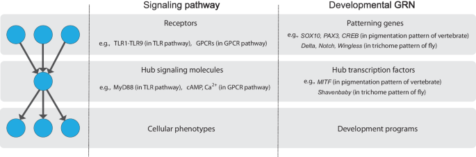
signaling networks9,10,11,12,13,14,15,16 (Fig. 1). For example, in the toll-like receptor (TLR) signaling network, various TLRs recognize pathogen-associated molecular patterns and the

signals are mediated through MyD88, resulting in the expression of various immune response genes14,16. In the G-protein coupled receptor (GPCR) signaling network, a vast number of GPCRs

encoded in the human genome primarily activate a few G proteins followed by the regulation of the calcium ion or cAMP concentration, which nonetheless lead to the induction of various gene

expressions causing diverse cellular phenotypes17,18,19. Bow-tie architecture is also found in the gene regulatory network. For example, in the gene regulatory network involved in the body

development, information from development patterning genes is integrated into the cis-regulatory region of the hub transcription factors, which regulates a large number of developmental

programs20,21,22. As distinct from these networks of information flow, bow-tie architecture is also found in the metabolic network that supports energy and material flow3,23. Bow-tie

architecture has also been reported in non-biological networks, such as internet protocols24,25 railroad transportation systems4, and so on. This universality of the bow-tie architecture

implies the existence of design principles underlying these systems, and thus it is important to elucidate how and why the bow-tie architecture emerges. Despite the ubiquity of bow-tie

architecture in living systems, the driving forces behind its emergence are still being debated. Kitano et al. have argued that bow-tie architecture is the result of optimization in the

trade-off among robustness, fragility, resource limitation, and performance1. Polouliakh et al. and Yan et al. have shown that a narrow intermediate layer in the bow-tie architecture

provides the capability to classify the inputs17,26. In terms of control theory, Wang et al. have proposed that bow-tie architecture possesses controllability27, and in line with this idea,

Kitano and Ni et al. have suggested that bow-tie architecture retains high evolvability, with a capacity for adjusting the outputs to the environment1,28. Although these studies have shown

the potential functions or advantages of bow-tie architecture, how this architecture evolved has not yet been elucidated. Friedlander et al. proposed an evolutionary mechanism of bow-tie

architecture based on their simulation using a linear network model2, in which the biological networks, specifically signaling networks, were modeled by a set of matrices describing the

network structure (Fig. 2a). They demonstrated that the bow-tie architecture emerges when (1) the mutations occur in a multiplicative manner, and (2) the network evolves toward a certain

target in-out relation (i.e., the goal matrix; see Fig. 2c) that is expressed by a rank-deficient matrix. The condition (1) models the characteristics of biological mutations in the

signaling network or gene regulatory network, which have been reported to be multiplicative29,30 and tend to minimize link intensity31. The condition (2) reflects biological inputs that are

often redundant32, such as image inputs in the retinal neural network31 or TLR signaling pathways33. Although this model assumes linear interaction for simplification, recent studies

reported that the linearity is observed at the level of the circuit in chemotactic signaling systems in animal networks34, suggesting that linear interaction can capture qualitative

behaviors and is not an inappropriate abstraction. A previous study2 proposed a clear formulation for addressing the bow-tie evolution and presented a plausible hypothesis. However, its

evolutionary dynamics remain unclear. In this study, we investigate a linear network model as a model of the signaling network, and report that bow-tie inevitably emerges regardless of goal

matrix rank in the early phase of evolution when link intensities representing molecular interactions are small in the initial conditions of evolutionary simulations. This indicates that the

network structure at the beginning of the evolution plays a crucial role in the emergence of bow-tie architecture. Furthermore, we analyzed the mechanism of the emergence of bow-tie

architecture by using a simple ODE model. Based on the identified mechanism of the emergence of bow-tie architecture, we also suggest that environmental fluctuation or an increase in the

number of input/output nodes, which is naturally considered in the biological evolution, facilitates the emergence of bow-tie architecture. Our study addresses the bow-tie architectures in

which information flow is transmitted through a few intermediate nodes, such as the architectures found in signal transduction and gene regulatory networks. Although bow-tie structure in

metabolic networks is also important, we exclude it from the scope of this study as the network of material flows with conservation laws makes the problem much more difficult. MODEL To

investigate the evolution of the bow-tie architecture, we consider layered feedforward networks with _M_ nodes in each layer. We adopted the linear network model proposed by ref. 2, in which

link intensities from the _l_th layer to the _l_ + 1 th layer are described by the _M_ × _M_ matrix \( {\bf A}^{{\boldsymbol{(}}l{\boldsymbol{)}}}\) (Fig. 2a). The \({ij}\) element,

\({A}_{{ij}}^{(l)}\), is the link intensity from node _j_ in the _l_th layer to node _i_ in the _l_ + 1 th layer and is defined as \({A}_{{ij}}^{(l)} \,>\, 0\). When an input signal _S_

is applied to the network with _L_ + 1 layers, output vector _V_ is obtained as the product of matrices \({\bf{As}}\,{\boldsymbol{=}}\,{\bf{v}}\), where \({\bf{A}}\) is the in-out relation

matrix of the network defined by \({{\bf{A}}\,=\,{\bf{A}}}^{(L)}{{\bf{A}}}^{(L-1)}...{{\bf{A}}}^{(1)}\) (Fig. 2a). A detailed explanation of the linear network model is given in

Supplementary Fig. 1. The network evolves toward an ideal in-out relation matrix _G_ (hereinafter referred to as the goal matrix) (Fig. 2b). We adopted a randomly generated goal matrix with

different ranks (Fig. 2c). The evaluation function, i.e., fitness, is defined by\(\,F=-\|{\bf{A}}-{\bf{G}}\|_{F}^{2}\), where the square of the Frobenius norm \(\|\cdot \|_{F}^{2}\)

represents the sum of the square of all matrix elements, and thus -\(F\) denotes the distance between the in-out relation matrix _A_ and the goal matrix _G_. We evolved the network by

optimizing the in-out relation matrix _A_ so that fitness \(F\) is maximized through the following genetic algorithm (Fig. 2b). We generate _N_ individuals having an _L_ + 1 layered network

represented by a set of matrices \({{\bf{A}}}^{(1)},\ldots ,{{\bf{A}}}^{(L)}\). In each generation during evolution, the individuals are duplicated so that the population size is 2 _N_ and

mutations are randomly introduced into 20% of individuals in that population. For the mutations, following Friedlander et al., we adopted the product rule mutation2 and a mutation rate of

0.2 per population, which is the same as the ref.2. A randomly selected network link \({A}_{{ij}}^{(l)}\) is altered as \({A}_{{ij}}^{(l)}\)→\({A}_{{ij}}^{(l)}\xi\) with a random number

\(\xi\) generated from \(N(1,\,0.1)\), i.e., a Gaussian distribution with mean one and variance 0.1. Variance 0.1 is selected to guarantee that \(\xi\) does not take a negative value but has

finite variance. Then, the fitness values _F_ for 2 _N_ individuals are evaluated, and finally the top _N_ individuals are selected by tournament selection with group size 42,31,35.

Evolution is simulated by repeating these processes (Fig. 2b). The individuals are considered to be fully evolved when their average fitness value reaches −0.01 or higher, and the network of

individuals with the highest fitness \({F}\) is analyzed. Throughout this study, the population size _N_ = 100 is used. Whether network architecture is bow-tie or not is judged by

calculating the decrease in fitness associated with the removal of each node. Deletion of node \(i\) at the _l_th layer is implemented by setting

\({A}_{{ik}}^{(l-1)}={A}_{{ki}}^{(l)}=0\,(k=\mathrm{1,2}\ldots M\,\)), and the absolute value of the associated fitness decrease is denoted by \(\Delta {F}_{i}^{l}\) (Fig. 2d). The ratio of

fitness decrease \({P}_{i}^{l}\) within _l_th layer is then estimated as \({P}_{i}^{l}=\frac{\Delta {F}_{i}^{l}}{{\sum }_{i}^{M}\Delta {F}_{i}^{l}}\). We define an active node as a node

whose removal causes a decrease in fitness satisfying a criterion \({P}_{i}^{l}\, >\) 0.001. When the number of the active nodes in a middle layer (i.e., the layer from _l_ = 2 to _L_ − 

1) is smaller than _M_, the network is defined as a bow-tie network. RESULTS BOW-TIE TRANSIENTLY EMERGES REGARDLESS OF GOAL WHEN INITIAL LINK INTENSITIES ARE SMALL First, we attempted to

reproduce the simulation of ref. 2. by using network of 6 nodes × 5 layers, i.e., _M_ = 6 and _L_ = 4 (Fig. 3a). We started the evolutionary simulation from a random configuration of

\({A}_{{ik}}^{(l)}\) with a small initial link intensity \({A}_{0}=0.01\), which is defined by the Frobenius norm of the initial in-out relation matrix \(\|{\bf{A}}\|_{F}\). We were able to

reproduce the previous results2, confirming that the network evolves to the bow-tie architecture when the goal matrix is rank-deficient (Fig. 3a). Although we adopted tournament selection

following the previous study2, we also confirmed that almost the same result was obtained by adopting elite selection (Supplementary Fig. 2). Figure 3a illustrates the most frequent number

of active nodes for each layer in the evolved network. We here refer to a middle layer with the smallest number of active nodes as a “waist” and denote its number of active nodes as the

“waist size”. The waist size decreases as the rank of the goal matrix decreases; for a low-rank goal matrix, the network with a narrow waist size evolves, while a network with a waist size =

 _M_ appears for the full-rank goal matrix (Fig. 3). We simulated the evolution of a network starting from various values of \({A}_{0}\). Figure 3b shows the waist size of the evolved

network against \({A}_{0}\), in which each dot represents the average value of over 100 runs, and illustrates that the bow-tie architecture evolves only at a range of \({A}_{0}\) (0.1–10).

This range is quite narrow compared with the Frobenius norm of the goal matrix, i.e., 60, denoted by the black dashed line in Fig. 3b. When we started the simulation with an \({A}_{0}\)

larger than 10, the network did not converge to a bow-tie structure in most cases (specifically for rank = 1). The probabilities for the bow-tie network with waist size = 1 exhibit a sharp

transition around \({A}_{0}\, \sim \,2.5\) as \({A}_{0}\) decreases, while the probabilities for the bow-tie with waist size <5 exhibit a transition around \({A}_{0}\)~ 10 in rank 1 and

gradual decreases in the ranks 2 and 3 (Supplementary Fig. 3a). The evolutionary dynamics also exhibited a remarkable dependence on initial link intensity \({A}_{0}\). Figure 3c shows the

time series of the number of active nodes in each layer for a large (=40) and small (=0.01) \({A}_{0}\) with different goal ranks. When the goal matrix was full-ranked, the number of the

active nodes in the 2–4th layers transiently decreased and then converged to 6 for the small \({A}_{0}\) (Fig. 3c; rank 6, solid black line), indicating a transient emergence of the bow-tie

architecture. For the large \({A}_{0}\), the number of active nodes did not show such a transient drop (Fig. 3c; rank 6, dashed black line). When the goal rank was low, the network starting

from the small \({A}_{0}\) converged to the bow-tie network (Fig. 3c; ranks 1–5, solid line), while the network starting from the large \({A}_{0}\) did not show even a transient emergence of

the bow-tie architecture (Fig. 3c; ranks 1–5, dashed line). Although the network shows different evolutionary trajectories that depend on the goal rank, the transient decrease of waist size

in the early phase of evolution can be observed in all ranks when evolution starts from the small \({A}_{0}\) (Fig. 3c and Supplementary Fig. 3b). Figure 3c elucidates that the waist width

takes a minimum value during a rapid increase in fitness (the bottom panels) and this transient bow-tie structure is maintained even after the fitness is almost saturated. This transient

emergence of bow-tie architecture was also confirmed for a larger network with 12 nodes × 5 layers (Supplementary Fig. 4) and for the other mutation rate (Supplementary Fig. 5). Figure 3d

shows the distribution of the instantaneous minimum waist size, which means the narrowest waist widths that the network reached during the course of evolution, and indicates that the network

transiently evolves to bow-tie architecture regardless of the rank of the goal matrix if it starts from a small \({A}_{0}\) (Fig. 3d; upper panel), while bow-tie architecture could not be

produced even in the low-rank goal matrix when the network started from a large \({A}_{0}\) (Fig. 3d; lower panel). The instantaneous minimum waist size as a function of \({A}_{0}\) shows

bow-tie emergence in the range of \({A}_{0} \sim 10\) in all ranks (Supplementary Fig. 3b). The transient emergence of bow-tie, and its dependence on the \({A}_{0}\), are also observed by

using the alternative active node definitions (i.e., the relative contribution of a node to the total in-out relation and relative value of the maximum interaction associated with a node;

see Methods and Supplementary Fig. 6). These results imply that bow-tie architecture can spontaneously emerge without low rank goal. The low-rank goal just determines whether or not the

transiently emerged bow-tie architecture is maintained. Furthermore, we also found that the bow-tie emergence weakly depends on the variance of goal matrix elements, as well as the initial

value \({A}_{0}\). Since the rank 1 goal has fewer independent elements than the rank 6 goal, the variance of the rank 1 goal tends to be smaller than that of the rank 6 goal. To eliminate

this bias, we normalized the variance and norm (see Methods and Supplementary Fig. 7). With this normalized goal, the condition of \({A}_{0}\) for the bow-tie emergence is more apparent as

\({0\, <\, A}_{0}\,\le\, 10\) (Supplementary Fig. 7a). Consistent with this finding, the probability for a bow-tie network with waist size <5 increases with decreasing _A_0 at _A_0 ≤ 

10 (Supplementary Fig. 7b). Most importantly, the transient emergence of the bow-tie network is completely independent of the goal rank (Supplementary Fig. 7c–e), which indicates that the

determinant of the bow-tie emergence is the initial value \({A}_{0}\) and the goal variances. ANALYSIS OF BOW-TIE ARCHITECTURE EVOLUTION BY THE DYNAMICAL SYSTEM To determine the reason for

the dependence on the initial link intensities \({A}_{0}\), we consider a phenomenological ordinary differential equation (ODE) of the network \({A}_{{ij}}^{\left(l\right)}\) that

qualitatively mimics the evolutionary simulation described above. Based on the gradient descent, the time evolution of link intensity \({A}_{{ij}}^{\left(l\right)}\) is given by

$$\frac{d{A}_{{ij}}^{\left(l\right)}}{{dt}}={\eta A}_{{ij}}^{\left(l\right)}\frac{\partial F}{\partial {A}_{{ij}}^{\left(l\right)}}{\boldsymbol{,}}$$ (1) where the product rule mutation is

implemented by the learning rate proportional to \({A}_{{ij}}^{\left(l\right)}\). This optimization algorithm, which we refer to here as the multiplicative gradient descent, describes the

multiplicative changes in the link intensity, and therefore the larger link changes more drastically. The learning rate \(\eta\) is set to a small constant value \(\eta \,={10}^{-4}\) to

avoid the computational instability. We confirmed that the results obtained using the ODE model (Supplementary Fig. 8) were almost the same as those by the original model (Fig. 3)—namely,

the ODE model reproduced bow-tie architectures for a rank-deficient goal matrix _G_ and a small \({A}_{0}\). We also confirmed that the ODE model exhibited a dependence on \({A}_{0}\)

similar to that of the original model (Supplementary Fig. 8a, b). The ODE model also recapitulated the transient appearance of the bow-tie in the original model (Supplementary Fig. 8c, d).

Using this ODE model, we here analyzed how the bow-tie architecture emerges in the early stage of the time evolution when starting from a small \({A}_{0}\). For simplicity, we consider

networks consisting of three layers with two nodes each (Supplementary Fig. 9a) with the most straightforward rank 1 goal matrix _G_ defined as _G_ = \(\left[\begin{array}{cc}g & g\\ g

& g\end{array}\right]\), where \(g\) takes an arbitrary positive value \(\left({g}\, >\, 0\,\right).\) The following argument can also be generalized for an arbitrary _G_ with rank 1

or rank 2 (Supplementary Note 2). Under this condition, the evaluation function is given as follows (Eq. 2):

$$F=-{\left\Vert{{\bf{A}}}^{\left(2\right)}{{\bf{A}}}^{\left(1\right)}-{\bf{G}}\right\Vert}_{F}^{2}=-{\rm{Tr}}\left[\left({{\bf{A}}}^{\left(2\right)}{{\bf{A}}}^{\left(1\right)}-{\bf{G}}\right){\left({{\bf{A}}}^{\left(2\right)}{{\bf{A}}}^{\left({1}\right)}-{\bf{G}}\right)}^{{\rm{T}}}\right]$$

(2) The adaptation process is modeled using the multiplicative gradient descent in Eq. (1) as follows (Supplementary Note 1):

$$\left\{\begin{array}{c}\displaystyle\frac{d}{{dt}}{{\bf{A}}}^{(2)}=-2\eta

\left[\left({{\bf{A}}}^{\left(2\right)}{{\bf{A}}}^{\left(1\right)}-{\bf{G}}\right){{\bf{A}}}^{\left(1\right),{\rm{T}}}\right]\odot {{\bf{A}}}^{\left(2\right)}\\

\displaystyle\frac{d}{{dt}}{{\bf{A}}}^{(1)}=-2\eta \left[{{\bf{A}}}^{\left(2\right),{\rm{T}}}\left({{\bf{A}}}^{\left(2\right)}{{\bf{A}}}^{\left(1\right)}-{\bf{G}}\right)\right]\odot

{{\bf{A}}}^{\left(1\right)}\end{array}\right.$$ (3) where \(\odot\) is the Hadamard product, i.e., \({({\bf{A}}\odot {\bf{B}})}_{{ij}}={a}_{{ij}}{b}_{{ij}}\), and

\({{\bf{A}}}^{\left(l\right),{\rm{T}}}\) is the transposed matrix of \({\bf A}^{\left(l\right)}\). Since we consider the early stage of the dynamics starting from

\({{\bf{A}}}^{\left(1\right)}\) and \({{\bf{A}}}^{\left(2\right)}\) that are much smaller than \({\bf{G}}\), the term

\(\left({{\bf{A}}}^{\left(2\right)}{{\bf{A}}}^{\left(1\right)}-{\bf{G}}\right)\) can be approximated as\(\,-{\bf{G}}\), and thus Eq. (3) is simplified as follows:

$$\frac{d}{{dt}}\left(\begin{array}{c}{{\bf{A}}}^{\left(2\right)}\\ {{\bf{A}}}^{\left(1\right),{\rm{T}}}\end{array}\right)=2\eta \left[\left(\begin{array}{cc}{\bf{0}} & {\bf{G}}\\

{{\bf{G}}}^{{\rm{T}}} & {\bf{0}}\end{array}\right)\left(\begin{array}{c}{{\bf{A}}}^{\left(2\right)}\\ {{\bf{A}}}^{\left(1\right),{\rm{T}}}\end{array}\right)\right]\odot

\left(\begin{array}{c}{{\bf{A}}}^{\left(2\right)}\\ {{\bf{A}}}^{\left(1\right),{\rm{T}}}\end{array}\right)$$ (4) By expanding Eq. (4), the following equation is obtained:

$$\frac{d}{{dt}}\left(\begin{array}{cc}\begin{array}{c}\begin{array}{c}{A}_{11}^{\left(2\right)}\\ {A}_{21}^{\left(2\right)}\end{array}\\ \begin{array}{c}{A}_{11}^{\left(1\right)}\\

{A}_{12}^{\left(1\right)}\end{array}\end{array} & \begin{array}{c}\begin{array}{c}{A}_{12}^{\left(2\right)}\\ {A}_{22}^{\left(2\right)}\end{array}\\

\begin{array}{c}{A}_{21}^{\left(1\right)}\\ {A}_{22}^{\left(1\right)}\end{array}\end{array}\end{array}\right)=2\eta

\left(\begin{array}{cc}\begin{array}{c}\begin{array}{c}g\left({A}_{11}^{\left(1\right)}+{A}_{12}^{\left(1\right)}\right){A}_{11}^{\left(2\right)}\\

g\left({A}_{11}^{\left(1\right)}+{A}_{12}^{\left(1\right)}\right){A}_{21}^{\left(2\right)}\end{array}\\

\begin{array}{c}g\left({A}_{11}^{\left(2\right)}+{A}_{21}^{\left(2\right)}\right){A}_{11}^{\left(1\right)}\\

g\left({A}_{11}^{\left(2\right)}+{A}_{21}^{\left(2\right)}\right){A}_{12}^{\left(1\right)}\end{array}\end{array} &

\begin{array}{c}\begin{array}{c}g\left({A}_{21}^{\left(1\right)}+{A}_{22}^{\left(1\right)}\right){A}_{12}^{\left(2\right)}\\

g\left({A}_{21}^{\left(1\right)}+{A}_{22}^{\left(1\right)}\right){A}_{22}^{\left(2\right)}\end{array}\\

\begin{array}{c}g\left({A}_{12}^{\left(2\right)}+{A}_{22}^{\left(2\right)}\right){A}_{21}^{\left(1\right)}\\

g\left({A}_{12}^{\left(2\right)}+{A}_{22}^{\left(2\right)}\right){A}_{22}^{\left(1\right)}\end{array}\end{array}\end{array}\right)$$ (5) Note that the first and second columns are

independent because the time evolution of \({({A}_{11}^{\left(2\right)},{A}_{21}^{\left(2\right)},{A}_{11}^{\left(1\right)},{A}_{12}^{\left(1\right)})}^{{\rm{T}}}\) does not depend on the

\({({A}_{12}^{\left(2\right)},{A}_{22}^{\left(2\right)},{A}_{21}^{\left(1\right)},{A}_{22}^{\left(1\right)})}^{{\rm{T}}}.\) The first column of Eq. (5) is given as

$$\frac{d}{{dt}}\left(\begin{array}{c}\begin{array}{c}{A}_{11}^{\left(2\right)}\\ {A}_{21}^{\left(2\right)}\end{array}\\ \begin{array}{c}{A}_{11}^{\left(1\right)}\\

{A}_{12}^{\left(1\right)}\end{array}\end{array}\right)=2\eta \left(\begin{array}{c}\begin{array}{c}g({A}_{11}^{\left(1\right)}+{A}_{12}^{\left(1\right)}){A}_{11}^{\left(2\right)}\\

g({A}_{11}^{\left(1\right)}+{A}_{12}^{\left(1\right)}){A}_{21}^{\left(2\right)}\end{array}\\ \begin{array}{c}g({A}_{11}^{\left(2\right)}+{A}_{21}^{\left(2\right)}){A}_{11}^{\left(1\right)}\\

g({A}_{11}^{\left(2\right)}+{A}_{21}^{\left(2\right)}){A}_{12}^{\left(1\right)}\end{array}\end{array}\right)$$ (6) Here, we define \({I}_{k}\) and \({R}_{k}\) as follows.

$$\begin{array}{c}{I}_{k}={A}_{k1}^{\left(1\right)}+{A}_{k2}^{\left(1\right)}\\ {R}_{k}={A}_{1k}^{\left(2\right)}+{A}_{2k}^{\left(2\right)}\end{array}$$ (7) \({I}_{k}\) represents the sum of

the input link intensities to the node _k_ in the middle layer, whereas \({R}_{k}\) denotes the sum of the output intensities from node _k_ in the middle layer (Supplementary Fig. 9a). From

Eqs. (6) and (7), the following relation holds: $$\begin{array}{c}\displaystyle\frac{d}{{dt}}{I}_{k}=2\eta g{R}_{k}{I}_{k}\\ \displaystyle\frac{d}{{dt}}{R}_{k}=2\eta

g{R}_{k}{I}_{k}\end{array}$$ (8) Thus, \(\frac{d}{{dt}}\left({R}_{k}-{I}_{k}\right)=0,\) indicating \({R}_{k}-{I}_{k}={R}_{k,0}-{I}_{k,0}\), where \({R}_{k.0}\) and \({I}_{k,0}\) are the

initial values of \({R}_{k}\) and \({I}_{k}\) (Supplementary Fig. 9b). Substituting this expression into Eq. (8), \(\frac{d}{{dt}}{R}_{k}\) is described as follows.

$$\frac{d}{{dt}}{R}_{k}=2\eta g{R}_{k}\left({R}_{k}-{R}_{k,0}+{I}_{k,0}\right)$$ (9) By solving this, the time evolution of \({R}_{k}\) is derived.

$${R}_{k}\left(t\right)=\frac{{R}_{k,0}\left({R}_{k,0}-{I}_{k,0}\right)}{{R}_{k,0}-{I}_{k,0}\exp \left[2\eta g\left({R}_{k,0}-{I}_{k,0}\right)t\right]}$$ (10) This indicates that \({R}_{k}\)

diverges within a finite time, \({t}=\frac{1}{2\eta g}\frac{\,\mathrm{ln}{R}_{k,0}-\mathrm{ln}{I}_{k,0}}{{R}_{k,0}-{I}_{k,0}}\), and \({I}_{k}\) also diverges since

\({R}_{k}-{I}_{k}={const}.\) The same argument holds for the second column of Eq. (5), since the equations for both columns are exactly symmetric and independent of each other. However, due

to the difference in the initial value, one of the two columns diverges prior to the other, and at this moment the network forms a bow-tie structure. Once this divergence of one of the two

columns occurs, the time evolution significantly slows down and the diverging nature in the dynamics vanishes since the assumption \({\bf{G}}-{\bf{A}}\,\approx\, {\bf{G}}\) does not hold,

which indicates that the transiently emerging bow-tie architecture is maintained. An example of the dynamics is shown in supplementary Fig. 9b, where \({R}_{1}\) and \({I}_{1}\) diverge

(Supplementary Fig. 9b; right panels) and accordingly, the bow-tie architecture associated with node 1 is formed (Supplementary Fig. 9b; left panels). For the case of \({R}_{k,0}\,\approx\,

{I}_{k,0}\), the divergent time is written as \(t \sim 1/g{R}_{k,0}\) (Supplementary Note 3), which indicates that the column that has a larger \({R}_{k,0}\) diverges first. Although the

rank 1 goal matrix with 2 nodes is assumed here, the independent relationships between columns of \(\left(\begin{array}{c}{{\bf{A}}}^{\left(2\right)}\\

{{\bf{A}}}^{\left(1\right),{\rm{T}}}\end{array}\right)\) in Eq. (4) hold, regardless of the goal matrix rank and number of nodes (Supplementary Note 2). Therefore, the bow-tie emergence with

the divergence of \(R\) and \(I\) for one of the columns always occurs if the approximation \({\bf{G}}-{\bf{A}}\,\approx\, {\bf{G}}\) is valid. The intuitive explanation for this effect is

as follows: In the case of \({\bf{G}}-{\bf{A}}\,\approx\, {\bf{G}}\), all \({A}_{{ij}}^{\left(l\right)}\) grow to increase the fitness, but the multiplicative nature of the growth leads to

the significant difference \({A}_{{ij}}^{\left(l\right)}\) among the _l_th layer; i.e., \({A}_{{ij}}^{\left(l\right)}\) starting from the smaller value grows more slowly, which causes the

bow-tie architecture. This is not the case for the condition under which the system starts from a large initial value \(\|{\bf{A}}\|_{F}\,\approx\, \|{\bf{G}}\|_{F}\), because the fitness

reaches the optimal value before the product rule mutation causes a significant difference of \({A}_{{ij}}^{\left(l\right)}\). These arguments help to explain how the bow-tie architecture

emerges in the early phase of evolution when the initial link intensities are small, regardless of the goal rank. ENVIRONMENTAL FLUCTUATION FACILITATES THE EMERGENCE OF THE BOW-TIE

ARCHITECTURE The aforementioned results assume a fixed goal matrix, which corresponds to the evolution under a fixed environment. However, in a more realistic situation, the elements of the

goal matrix (ideal in-out relation) fluctuate due to the environmental fluctuation or mutations in the numbers of the receptors and downstream genes. To examine the effect of an

environmental fluctuation on the evolution of bow-tie architecture, we introduced the variable goal matrix without changing the dimension, rank, or norm. First, the network evolves under the

first goal matrix for 150,000 generations, which is enough time for the fitness to reach 0.01. Second, the goal matrix is altered to the next one. We found that the network architectures

are maintained irrespective of any such change in the goal matrix during evolution; the waist width did not change between before and after the change in goal matrix (Supplementary Fig. 10),

indicating that the waist width is not affected by the change in goal matrix but determined by \({A}_{0}\). The number of active nodes transiently increases immediately after the change of

goal matrix. This is attributed to the definition of active nodes; due to the decrease in fitness associated with the change in the goal matrix, the difference of \(\Delta {F}_{i}^{l}\)

(i.e., the fitness decrease by the _l_th node removal) among nodes in the _l_th layer is less clear, and thus the value of \({P}_{i}^{l}=\Delta {F}_{i}^{l}/{\sum }_{i}^{M}\Delta

{F}_{i}^{l}\) tends to exceed the threshold, which leads to an increase in the waist width. These results reflect that the bow-tie architectures are robust to environmental fluctuations that

do not alter the rank and norm once the bow-tie architecture emerges. Consistent with such a conclusion, after the network adapts to the initial goal, the network architecture does not

change by repeated changes in the goal matrix. Figure 4a shows the time-course of the active nodes in each layer during the repeated goal change with a fixed goal rank (ranks 1 and 6) every

1000 generations, indicating that the network architecture is maintained (for ranks 2 and 3, see Supplementary Fig. 11a). Interestingly, after the adaptation to the goal matrix, the network

structure is still maintained even for the changes in the rank of the goal matrix. The network is first evolved to adapt to the rank 1 goal, and then the goal matrix is repeatedly switched

to the randomly generated full-rank goal matrix every \({10}^{3}\) generation (Fig. 4b). This procedure did not change the bow-tie architecture during \({10}^{4}\) generations. Similarly,

the retention of bow-tie architecture was also observed in the changes from rank 2 to rank 6 and from rank 3 to rank 6 (Supplementary Fig. 11b). Although these data indicate that the

environmental fluctuation does not affect the previously emerged bow-tie architecture, this is not the case when the fluctuation takes place at the beginning of the evolution. When starting

from a small initial link intensity \({A}_{0}\) (\({A}_{0}=0.01\)), the initial random network develops the bow-tie architecture by the repeated fluctuation of the goal matrix, regardless of

the goal rank (Fig. 4c and Supplementary Fig. 11c). This can be understood by the fact that the time-averaged goal matrix can be effectively interpreted as a rank 1 matrix, which

facilitates the bow-tie emergence. GENE DUPLICATION ACCELERATES THE EMERGENCE OF THE BOW-TIE ARCHITECTURE We next examined the effect of the expansion of the goal matrix. During evolution,

the number of the input and output nodes can be increased by gene duplication, and by de-novo addition (emergence) of the receptor molecules and downstream genes. Therefore, we investigated

whether the non-bow-tie network switches to the bow-tie architecture in response to an increase in the goal matrix dimension. We found that an increase in the goal matrix dimension indeed

leads to the emergence of the bow-tie architecture even when starting from a large link intensity (Fig. 5). The details of the simulation procedure are shown in Fig. 5a: Evolutionary

simulations were started from a network including 10 nodes by 5 layers with a large initial link intensity (\({{\rm{A}}}_{0}=10)\) under a rank 1 goal. Since the simulation started from a

large \({{\rm{A}}}_{0}\), the network did not evolve to a bow-tie network. Nevertheless, by expanding the goal matrix from a 10 × 10 matrix to a 20 × 20 matrix at the 1000th generation (Fig.

5a), the waist width was reduced, resulting in the convergence (|Fitness| < 0.01) to the bow-tie architecture with a narrower waist (Fig. 5b,c). Note that although the input and output

nodes are increased by the goal matrix expansion, the evolved waist width is lower than that before expanding the goal matrix (Fig. 5c, d). This would also be explained from the proposed

scenario starting from a small link intensity; the expansion of the goal matrix results in the increase in the norm of the goal matrix \({\bf{G}},\) causing\(\,\|{\bf{G}}\|_{F}\gg

\|{\bf{A}}\|_{F}\), and subsequently leads to evolution of the bow-tie architecture as discussed in the above section. BOW-TIE NETWORK WITH NON-LINEAR INTERACTIONS Although we considered a

network with linear interactions in this study, actual biological interactions are often non-linear. Hence, we examined whether the bow-tie architecture emerges in the \({A}_{0}\) dependent

manner even when the interactions are non-linear. In a non-linear network, the activation function \(f\left(x\right)=(1+\tanh ({\rm{x}}))/2\) is introduced into each layer. The network

evolves to solve a classification task of the 64-bit image of a handwritten digit. The input \({\bf{v}}\) is a 64-length array that represents the 2D (8×8) image of a handwritten number (the

digit dataset in scikit-learn). The handwritten numbers in the input images are “2”, “4”, “6” and “8”, and these images are classified into the redundant six groups (see Supplementary Fig.

13a), which is encoded to a 6-bit array of the output. The network consists of 5 layers (64 nodes for the input layer and 6 nodes for the other layers). The network output is described as

\({\bf{u}}={f}({\bf{A}}^{\left(4\right)}f({\bf{A}}^{\left(3\right)}{{f}({\bf{A}}}^{\left(2\right)}f({{\bf{A}}}^{\left(1\right)}{\bf{v}})))\), where \({\bf{u}}\) and \({\bf{v}}\) are the

output and input vectors, while \({\bf{A}}^{(1)}\in {R}_{6\times 64}\) and \({\bf{A}}^{\left(i\right)}\in {R}_{6\times 6},{i}={2,3,4}\) (Supplementary Fig. 13a). By genetic algorithm with

the multiplicative mutations, the network was trained to solve the classification problem for the image inputs (300 images). In the initial condition, \({A}_{{ij}}^{\left(l\right)}\) is

extracted from the uniform distribution from −1 to 1, followed by the normalization of the norm of

\({\bf{A}}={\bf{A}}^{\left(4\right)}{\bf{A}}^{\left(3\right)}{\bf{A}}^{\left(2\right)}{\bf{A}}^{\left(1\right)}\) to \({A}_{0}\). The mutation size is set to large so that the intensities

can take both negative and positive values (i.e., \(\xi \sim N(1,\,0.5)\)). Supplementary Fig. 13b shows the time trajectory of the number of the active nodes in each layer. The networks

starting from small link intensities \({A}_{0}\) (Supplementary Fig. 13b: solid line) tended to have a narrower middle layer in both the transient and end state than those starting from a

large \({A}_{0}\) (Supplementary Fig. 13b: dashed line). This suggests that the initial value plays a crucial role in the evolution of bow-tie architecture, even in a non-linear network.

DISCUSSION In this study, we investigated the conditions under which the bow-tie architecture emerges by using an evolutionary simulation with a linear network model. We found that the prime

determinant of the bow-tie emergence is the link intensity of the initial network \({A}_{0}\) rather than characteristics in the goal matrix. In the end state of evolution, only when

evolution starts from small \({A}_{0}\), the network can evolve into a bow-tie architecture in a goal matrix rank-dependent manner. In the transient state of evolution, when evolution starts

from small \({A}_{0}\), bow-tie architecture always emerges independently from the goal matrix rank. Namely, the bow-tie emerges spontaneously when \({A}_{0}\) is small, and the rank of the

goal matrix determines whether or not the transiently emerged bow-tie will be maintained until the end state. From the analysis using the ODE model (Fig. 4), we concluded that this

emergence of bow-tie architecture is attributable to the growth from a small value of \({A}_{0}\) with the multiplicative nature of the increase in \({A}_{{ij}}^{\left(l\right)}\), which can

cause the significant differences in \({A}_{{ij}}^{\left(l\right)}\) among the _l_th layers. Our result indicates that the initial value plays a crucial role in the evolution of bow-tie

architecture rather than the goal matrix, which was overlooked in the previous study2. The evolution from small \({A}_{0}\) (i.e., small link intensity) may correspond to the early stage in

the evolution, where molecular interactions are almost entirely absent. Consistent with such an assumption that the bow-tie network could emerge at the early stage of the evolution, a core

of the bow-tie architecture is well conserved (e.g., G proteins), implying that the architecture has a very old origin19,36,37. On the other hand, the evolution from a large \({A}_{0}\)

corresponds to a readapting after the network evolves to a non-bow-tie architecture. In this case, under a new goal, the network does not attain a bow-tie structure unless the condition

\(\|{\bf{G}}\|_{F}\gg {A}_{0}\) is satisfied for the new goal. For the case with \(\|{\bf{G}}\|_{F}\gg {A}_{0}\), the bow-tie architecture emerges after the goal matrix changes to the large

norm goal matrix (Fig. 5). It is known that the bow-tie architecture is robust against perturbation1,2,23 and thus the core is well conserved19,36,37. Consistent with these facts, we

confirmed that once the bow-tie architecture is established, it is robust against the goal matrix fluctuations (Fig. 4a, b). Additionally, we found that continuous change of the goal matrix

stabilizes the bow-tie architecture (Fig. 4c). The vast number of inputs and outputs is also characteristic of bow-tie architecture. Thus we examined the relationship between the expansion

event of input/output (i.e., genome duplication, de novo addition) and bow-tie evolution. We found that a sudden increase in the number of inputs and outputs narrowed the waist width in the

network, leading to the bow-tie architecture, even though the adaptation process started from a relatively large initial condition. In addition, the previous study2 showed that once a

bow-tie architecture is established, it is robust to further goal matrix expansion (Supplementary Fig. 17 in ref. 2). Similarly, information processing has been reported to be robust against

the increase in input/output nodes38. These findings suggest that the addition of inputs and outputs (i.e., goal matrix expansion) does not disturb the bow-tie structure, and can even

promote its emergence (Fig. 5). In fact, in the GPCR signaling system, which forms a narrow waist bow-tie architecture, the numbers of receptors and downstream genes have been reported to

increase rapidly36,39. However, further analysis will be needed to determine whether such expansion gave rise to the formation of bow-tie architecture in actual biological systems. It is

also important to address how the size of the intermediate layer grows as the network size increases and to examine the presence or absence of the scaling law in these growth curves, as was

observed in the archaea genome40. Our results indicate that the bow-tie architecture can emerge in a goal-independent manner. This suggests a possibility that the bow-tie architecture

emerges as a byproduct of evolution, where a phenotype can emerge regardless of the evolutionary goal. However, it does not deny the possibility that the bow-tie architecture emerges as the

result of selection for the functional advantages suggested by the previous studies17,26,27,28 or as the result of the rank-deficient task2. For example, the bow-tie architecture can be

controlled by controlling input signals27, and it shows fast adaptation to novel environments and high evolvability 28. Such fast adaptation of the bow-tie architecture was also seen in our

simulation (Fig. 4a, red line in the bottom panel). We also found that the network generally evolves to a bow-tie architecture under the fluctuating goal matrix (Fig. 4c and Supplementary

Fig. 11c). This suggests that the bow-tie structure can provide a fast adaptation to a fluctuating environment. On the other hand, the bow-tie network has a high lethality to perturbation to

the core nodes41,42 and is disadvantageous for use in a search for alternative core genes23. The bow-tie architecture would have been selected as the result of a trade-off between these

advantages and disadvantages23. The cost of having interactions could also promote the bow-tie structure. For example, when the cost of the L1 regularization term \(\lambda \mathop{\sum

}\limits_{l=1}^{L}\mathop{\sum }\limits_{i,j=1}^{M}|{A}_{{ij}}^{(l)}|\) is included in the fitness, the networks evolve towards the bow-tie architecture (Supplementary Fig. 12) independent

of the initial link intensities _A__0_, while the cost of the L2 regularization term \(\lambda \mathop{\sum }\limits_{l=1}^{L}\mathop{\sum

}\limits_{i,j=1}^{M}{\left({A}_{{ij}}^{(l)}\right)}^{2}\) cannot enhance the bow-tie structure (Supplementary Fig. 12). These results are explainable by the well-known effect in the data

sciences43 that the L1 regularization term reduces the network links. However, it is not obvious whether the cost for \({A}_{{ij}}\) can be approximated by L1, L2 or other types of

regularization. Thus, it would be important to consider a cost-independent scenario, as was demonstrated in this study. Bow-tie architecture is also closely related to the neural network.

The linear network model that we adopted corresponds to a neural network with a linear activation function. Even in this linear model, behaviors analogous to widely used neural networks have

been reported44,45. The evolutionary simulation of a non-linear network performed herein (Supplementary Fig. 13) corresponds to an image classification by a genetic algorithm-optimized

neural network. Further, neural networks incorporating bottlenecks in the hidden layers, such as VAE (Variational Autoencoder), are employed for tasks such as dimension reduction. Thus, a

comparison of neural networks and the biological bow-tie architecture might yield interesting insights. For example, from this aspect, the information-theoretic principle38 and

classification ability17 have been evaluated in signaling pathways. In summary, we found that a key determinant of the bow-tie emergence is the intensity of molecular interactions,

\({A}_{0}\), at the initial stage of the evolution, and the bow-tie structure appears if the mathematical condition\(\,\|{\bf {G}}\|_{{\rm{F}}}\gg {A}_{0}\) (i.e., a large gap between the

initial and goal link intensities) is satisfied. This condition would hold in (1) the early stage of evolution and (2) evolution after an addition of input and output nodes. Furthermore, the

transiently appearing bow-tie structure is maintained under a fluctuating evolutionary goal. Although a feedforward network was adopted here, a more realistic interaction including feedback

loops should be examined in the future. Finally, a bioinformatic analysis revealing the origin and evolutionary history of bow-tie architecture will be required to support our hypothesis.

METHODS THE DEFINITIONS OF THE ACTIVE NODE In our simulation, we mainly used the definition of the active node based on the relative fitness contribution (the 1st definition below), while we

also confirmed that the obtained results do not change by using other definitions of the active node, such as that based on the relative contribution to the total in-out relation (the 2nd

definition below), and that based on the relative strength of maximal interaction (the 3rd definition below). The details of the definitions of the active nodes are as follows: RELATIVE

CONTRIBUTION OF EACH NODE TO THE FITNESS The active nodes are determined by evaluating the following \({P}_{i}^{l}\) for all nodes: $${P}_{i}^{l}=\frac{{{\rm{||}}\Delta

{F}_{i}^{l}{\rm{||}}}_{F}^{2}}{{\sum }_{j}^{M}{{||}\Delta {F}_{j}^{l}{||}}_{F}^{2}}$$ (11) where \(\Delta {F}_{i}^{l}\) is a fitness decrease by the deletion of the node \(i\) in layer

\(l\). The node that shows \({P}_{i}^{l}\, >\, 0.001\) is categorized as the active node. RELATIVE CONTRIBUTION OF EACH NODE TO THE TOTAL IN-OUT RELATION The active nodes are determined

by evaluating the following \({P}_{i}^{l}\) for all nodes: $${P}_{i}^{l}=\frac{{{\rm{||}}{{\Delta }}{{\bf{A}}}_{i}^{l}{\rm{||}}}_{F}^{2}}{{\sum }_{j}^{M}{{\rm{||}}\Delta

{{\bf{A}}}_{j}^{l}{\rm{||}}}_{F}^{2}}$$ (12) where \(\Delta {{\bf{A}}}_{i}^{l}={\bf{A}}-\,{{\bf{A}}}_{{\rm{del}},{i}}^{l}\,\). \({{\bf{A}}}_{{\rm{del}},{i}}^{l}\) is a total in-out relation

when node \(i\) in layer \(l\) is deleted. The node that shows \({P}_{i}^{l}\, >\, 0.001\) is categorized as the active node. RELATIVE STRENGTH OF MAXIMAL INTERACTION OF EACH NODE The

active nodes are determined by evaluating the following \({P}_{i}^{l}\) for all nodes: $${P}_{i}^{l}=\frac{{m}_{i}^{l}}{{\sum }_{j}^{M}{m}_{j}^{l}}$$ (13) where \({m}_{i}^{l}\) describes the

maximum interactions associated with node \(i\) among inputs \({A}_{{ik}}^{l-1}\) and outputs \({A}_{{ki}}^{l}\), i.e., \({m}_{i}^{l}=\max ({A}_{i1}^{l-1},\ldots

,{A}_{{iM}}^{l-1},\,{A}_{1i}^{l},\ldots ,{A}_{{Mi}}^{l})\). The node that shows \({P}_{i}^{l}\, >\, 0.05\) is categorized into the active node. GOAL MATRIX NORMALIZATION OF VARIANCE AND

NORM The normalization of the variance and norm of each of the elements in the \(N\times N\) goal matrix is performed using the following equation:

$${Z}_{{ij}}=\,\frac{{G}_{{ij}}-\,{\boldsymbol{ < }}\,{G}_{{ij}}{\boldsymbol{ > }}}{\sqrt{{V}_{{G}_{{ij}}}}}+\,\sqrt{\frac{D}{{N}^{2}}-\,1},$$ (14) where \({\boldsymbol{ <

}}\,{G}_{{ij}}{\boldsymbol{ > }}\) is the average of elements in matrix _G_ defined by \({\boldsymbol{ < }}{G}_{{ij}}{\boldsymbol{ > }}\,{\boldsymbol{=}}\,\frac{1}{{N}^{2}}{\sum

}_{i}^{N}{\sum }_{j}^{N}{G}_{{ij}}\), while \({V}_{{G}_{{ij}}}\) is the variance of elements defined by \({V}_{{G}_{{ij}}}=\frac{1}{{N}^{2}}{\sum }_{i}^{N}{\sum }_{j}^{N}{\left({G}_{{ij}}-

< {G}_{{ij}} > \right)}^{2}\). Goal matrix _G_ is a random matrix with arbitrary rank. The normalized goal matrix _Z_ shows variance \({V}_{{Z}_{{ij}}}=1\) and norm

\(\|{\bf{Z}}\|_{F}^{2}=D\) as shown in the following derivation. Variance: $${V}_{{Z}_{{ij}}}=\frac{1}{{N}^{2}}\mathop{\sum }\limits_{i}^{N}\mathop{\sum }\limits_{j}^{N}{\left({Z}_{{ij}}-

<\, {Z}_{{ij}}\, > \right)}^{2}=\frac{1}{{{V}_{{G}_{{ij}}}N}^{2}}\mathop{\sum }\limits_{i}^{N}\mathop{\sum }\limits_{j}^{N}{\left({G}_{{ij}}-\, < {G}_{{ij}}\, > \right)}^{2}=1.$$

(15) Norm: $$\begin{array}{c}{{{||}}{\bf{Z}}{{||}}}_{F}^{2}=\mathop{\sum }\limits_{i}^{N}\mathop{\sum }\limits_{j}^{N}{{Z}_{{ij}}}^{2}={N}^{2}(V_{{Z}_{{ij}}}+\,{ <\, {Z}_{{ij}}\, >

}^{2})\\\quad\; ={N}^{2}\left(1+\,{\left(\sqrt{\displaystyle\frac{D}{{N}^{2}}-1}.\right)}^{2}\right)=D,\end{array}$$ (16) where \(<\, {{Z}_{{ij}}}^{2}\, > =\,{V}_{{Z}_{{ij}}}+\,{

<\, {Z}_{{ij}}\, > }^{2}\) is used. DATA AVAILABILITY All data used in this study can be freely downloaded from Zenodo (https://doi.org/10.5281/zenodo.11090260). CODE AVAILABILITY Code

files are freely available from the GitHub repository (https://github.com/itotoma/BowTie_evolution.git). REFERENCES * Kitano, H. Biological robustness. _Nat. Rev. Genet._ 5, 826–837 (2004).

Article  CAS  PubMed  Google Scholar  * Friedlander, T., Mayo, A. E., Tlusty, T. & Alon, U. Evolution of bow-tie architectures in biology. _PLoS Comput. Biol._ 11, e1004055 (2015).

Article  PubMed  PubMed Central  Google Scholar  * Doyle, J. C. & Csete, M. Architecture, constraints, and behavior. _Proc. Natl Acad. Sci. USA_ 108, 15624–30 (2011). Article  CAS 

PubMed  PubMed Central  Google Scholar  * Tieri, P. et al. Network, degeneracy and bow tie. Integrating paradigms and architectures to grasp the complexity of the immune system. _Theor.

Biol. Med. Model._ 7, 32 (2010). Article  PubMed  PubMed Central  Google Scholar  * Ma, H. W. & Zeng, A. P. The connectivity structure, giant strong component and centrality of metabolic

networks. _Bioinformatics_ 19, 1423–30 (2003). Article  CAS  PubMed  Google Scholar  * Ma, H. et al. The Edinburgh human metabolic network reconstruction and its functional analysis. _Mol.

Syst. Biol._ 3, 135 (2007). Article  PubMed  PubMed Central  Google Scholar  * Yang, R., Zhuhadar, L. & Nasraoui, O. Bow-tie decomposition in directed graphs. In _Proc.14th International

Conference on Information Fusion._ 1–5 (IEEE, 2011). * Ghosh, R. G., He, S., Geard, N. & Verspoor, K. Bow-tie architecture of gene regulatory networks in species of varying complexity.

_J. R. Soc. Interface._ 18, 179 (2021). Google Scholar  * Natarajan, M., Lin, K. M., Hsueh, R. C., Sternweis, P. C. & Ranganathan, R. A global analysis of cross-talk in a mammalian

cellular signalling network. _Nat. Cell. Biol._ 8, 571–80 (2006). Article  CAS  PubMed  Google Scholar  * Behar, M. & Hoffmann, A. Understanding the temporal codes of intra-cellular

signals. _Curr. Opin. Genet. Dev._ 20, 684–93 (2010). Article  CAS  PubMed  PubMed Central  Google Scholar  * Jordan, J. D., Landau, E. M. & Iyengar, R. Signaling networks: the origins

of cellular multitasking. _Cell_ 103, 193–200 (2000). Article  CAS  PubMed  PubMed Central  Google Scholar  * Nelson, M. D. et al. A bow-tie genetic architecture for morphogenesis suggested

by a genome-wide RNAi screen in Caenorhabditis elegans. _PLoS genet_ 7, e1002010 (2011). Article  CAS  PubMed  PubMed Central  Google Scholar  * Abd-Rabbo, D. & Michnick, S. W.

Delineating functional principles of the bow tie structure of a kinase-phosphatase network in the budding yeast. _BMC Syst. Biol._ 11, 38 (2017). Article  PubMed  PubMed Central  Google

Scholar  * Supper, J. et al. BowTieBuilder: modeling signal transduction pathways. _BMC Syst. Biol._ 3, 67 (2009). Article  PubMed  PubMed Central  Google Scholar  * Beutler, B. Inferences,

questions and possibilities in toll-like receptor signalling. _Nature_ 430, 257–63 (2004). Article  CAS  PubMed  Google Scholar  * Oda, K. & Kitano, H. A comprehensive map of the

toll-like receptor signaling network. _Mol. Syst. Biol._ 2, 2006.0015 (2006). Article  PubMed  PubMed Central  Google Scholar  * Polouliakh, N., Nock, R., Nielsen, F. & Kitano, H.

G-protein coupled receptor signaling architecture of mammalian immune cells. _PLoS One_ 4, e4189 (2009). Article  PubMed  PubMed Central  Google Scholar  * Oda, K., Matsuoka, Y., Funahashi,

A. & Kitano, H. A comprehensive pathway map of epidermal growth factor receptor signaling. _Mol. Syst. Biol._ 1, 2005.0010 (2005). Article  PubMed  PubMed Central  Google Scholar  *

Mendoza, A. D., Sebé-Pedrós, A. & Ruiz-Trill, I. The evolution of the GPCR signaling system in eukaryotes: modularity, conservation, and the transition to metazoan multicellularity.

_Genome Biol. Evol._ 6, 606–619 (2014). Article  PubMed  PubMed Central  Google Scholar  * Stern, D. L. & Orgogozo, V. Is genetic evolution predictable? _Science_ 323, 746–51 (2009).

Article  CAS  PubMed  PubMed Central  Google Scholar  * Mann, R. S. & Carroll, S. B. Molecular mechanisms of selector gene function and evolution. _Curr. Opin. Genet. Dev._ 12, 592–600

(2002). Article  CAS  PubMed  Google Scholar  * Kopp, A. Metamodels and phylogenetic replication: a systematic approach to the evolution of developmental pathways. _Evolution_ 63, 2771–89

(2009). Article  PubMed  Google Scholar  * Csete, M. & Doyle, J. C. Bow ties, metabolism and disease. _Trends Biotechnol._ 22, 446–50 (2004). Article  CAS  PubMed  Google Scholar  *

Akhshabi, S. & Dovrolis, C. The evolution of layered protocol stacks leads to an hourglass-shaped architecture. _SIGCOMM Comput. Commun. Rev._ 41, 206 (2011). Article  Google Scholar  *

Broder, A. et al. Graph structure in the web. _Comput. Netw._ 33, 309–320 (2000). Article  Google Scholar  * Yan, J. et al. Bow-tie signaling in c-di-GMP: machine learning in a simple

biochemical network. _PLoS Comput. Biol._ 13, e1005677 (2017). Article  PubMed  PubMed Central  Google Scholar  * Wang, D., Jin, S. & Zou, X. Crosstalk between pathways enhances the

controllability of signalling networks. _IET Syst. Biol._ 10, 2–9 (2016). Article  PubMed  PubMed Central  Google Scholar  * Ni, B. et al. Evolutionary remodeling of bacterial motility

checkpoint control. _Cell Rep._ 18, 866–877 (2017). Article  CAS  PubMed  PubMed Central  Google Scholar  * Wells, J. A. Additivity of mutational effects in proteins. _Biochemistry_ 29,

8509–17 (1990). Article  CAS  PubMed  Google Scholar  * Maerkl, S. J. & Quake, S. R. A systems approach to measuring the binding energy landscapes of transcription factors. _Science_

315, 233–7 (2007). Article  CAS  PubMed  Google Scholar  * Friedlander, T., Mayo, A. E., Tlusty, T. & Alon, U. Mutation rules and the evolution of sparseness and modularity in biological

systems. _PLoS One_ 8, e70444 (2013). Article  CAS  PubMed  PubMed Central  Google Scholar  * Tong, A. H. et al. Systematic genetic analysis with ordered arrays of yeast deletion mutants.

_Science_ 294, 2364–8 (2001). Article  CAS  PubMed  Google Scholar  * Chauhan, P., Shukla, D., Chattopadhyay, D. & Saha, B. Redundant and regulatory roles for Toll-like receptors in

Leishmania infection. _Clin. Exp. Immunol._ 190, 167–186 (2017). Article  CAS  PubMed  PubMed Central  Google Scholar  * Nunns, H. & Goentoro, L. Signaling pathways as linear

transmitters. _Elife_ 7, e33617 (2018). Article  PubMed  PubMed Central  Google Scholar  * Katoch, S., Chauhan, S. S. & Kumar, V. A review on genetic algorithm: past, present, and

future. _Multimed. Tools Appl._ 80, 8091–8126 (2021). Article  PubMed  Google Scholar  * Huang, Y., Zheng, Y., Su, Z. & Gu, X. Differences in duplication age distributions between human

GPCRs and their downstream genes from a network prospective. _BMC Genom._ 10, S14 (2009). Article  Google Scholar  * Vallabhajosyula, R. R., Chakravarti, D., Lutfeali, S., Ray, A. &

Raval, A. Identifying hubs in protein interaction networks. _PLoS One_ 4, e5344 (2009). Article  PubMed  PubMed Central  Google Scholar  * Hilliard, S. et al. Bow-tie architectures in

biological and artificial neural networks: implications for network evolution and assay design. _iScience_ 26, 106041 (2023). Article  CAS  PubMed  PubMed Central  Google Scholar  * Hwang,

J. I. et al. Expansion of secretin-like G protein-coupled receptors and their peptide ligands via local duplications before and after two rounds of whole-genome duplication. _Mol. Biol.

Evol._ 30, 1119–30 (2013). Article  CAS  PubMed  Google Scholar  * Van, N. E. Scaling laws in the functional content of genomes. _Trends Genet._ 19, 479–84 (2003). Article  Google Scholar  *

He, X. & Zhang, J. Why do hubs tend to be essential in protein networks? _PLoS Genet._ 2, e88 (2006). Article  PubMed  PubMed Central  Google Scholar  * Jeong, H., Mason, S. P.,

Barabási, A. L. & Oltvai, Z. N. Lethality and centrality in protein networks. _Nature_ 411, 41–2 (2001). Article  CAS  PubMed  Google Scholar  * Rish, I. & Grabarnik, G. _Sparse

Modeling: Theory, Algorithms, and Applications_, 109 (CRC Press, 2014). * Saxe, A. M., McClelland, J. L. & Ganguli, S. Exact solutions to the nonlinear dynamics of learning in deep

linear neural networks, (2014). arXiv:1312.6120v3. * Saxe, A. M., McClelland, J. L. & Ganguli, S. A mathematical theory of semantic development in deep neural networks. _Proc. Natl Acad.

Sci. USA_ 116, 11537–11546 (2019). Article  CAS  PubMed  PubMed Central  Google Scholar  Download references ACKNOWLEDGEMENTS We thank all members of the Aoki Laboratory for the helpful

discussion. This study was supported in part by the Cooperative Study Program of the Exploratory Research Center on Life and Living Systems (ExCELLS; programs no. 21-102 and 22-102 to

N.S.)and the Japan Society for the Promotion of Science (KAKENHI grants no. 19H05675 to Y.K., 23KJ1009 to T.I., and 23H04316 to N.S.). AUTHOR INFORMATION AUTHORS AND AFFILIATIONS * National

Institute for Basic Biology, National Institutes of Natural Sciences, 5-1 Higashiyama, Myodaiji-cho, Okazaki, Aichi, 444-8787, Japan Thoma Itoh, Yohei Kondo & Kazuhiro Aoki * Department

of Basic Biology, School of Life Science, SOKENDAI (The Graduate University for Advanced Studies), 5-1 Higashiyama, Myodaiji-cho, Okazaki, Aichi, 444-8787, Japan Thoma Itoh, Yohei Kondo 

& Kazuhiro Aoki * Exploratory Research Center on Life and Living Systems (ExCELLS), National Institutes of Natural Sciences, 5-1 Higashiyama, Myodaiji-cho, Okazaki, Aichi, 444-8787,

Japan Thoma Itoh, Yohei Kondo, Kazuhiro Aoki & Nen Saito * Graduate School of Integrated Sciences for Life, Hiroshima University, Higashihiroshima, Hiroshima, 739-8511, Japan Nen Saito

Authors * Thoma Itoh View author publications You can also search for this author inPubMed Google Scholar * Yohei Kondo View author publications You can also search for this author inPubMed 

Google Scholar * Kazuhiro Aoki View author publications You can also search for this author inPubMed Google Scholar * Nen Saito View author publications You can also search for this author

inPubMed Google Scholar CONTRIBUTIONS Conceptualization: T.I., Y.K., K.A., and N.S. Supervision: Y.K., K.A., and N.S. Investigation: T.I. Methodology: T.I. and N.S. Writing: T.I. and N.S.

All authors approved the final manuscript. CORRESPONDING AUTHOR Correspondence to Nen Saito. ETHICS DECLARATIONS COMPETING INTERESTS The authors declare no competing interests. ADDITIONAL

INFORMATION PUBLISHER’S NOTE Springer Nature remains neutral with regard to jurisdictional claims in published maps and institutional affiliations. SUPPLEMENTARY INFORMATION SUPPLEMENTARY

MATERIAL RIGHTS AND PERMISSIONS OPEN ACCESS This article is licensed under a Creative Commons Attribution 4.0 International License, which permits use, sharing, adaptation, distribution and

reproduction in any medium or format, as long as you give appropriate credit to the original author(s) and the source, provide a link to the Creative Commons licence, and indicate if changes

were made. The images or other third party material in this article are included in the article’s Creative Commons licence, unless indicated otherwise in a credit line to the material. If

material is not included in the article’s Creative Commons licence and your intended use is not permitted by statutory regulation or exceeds the permitted use, you will need to obtain

permission directly from the copyright holder. To view a copy of this licence, visit http://creativecommons.org/licenses/by/4.0/. Reprints and permissions ABOUT THIS ARTICLE CITE THIS

ARTICLE Itoh, T., Kondo, Y., Aoki, K. _et al._ Revisiting the evolution of bow-tie architecture in signaling networks. _npj Syst Biol Appl_ 10, 70 (2024).

https://doi.org/10.1038/s41540-024-00396-8 Download citation * Received: 15 January 2024 * Accepted: 14 June 2024 * Published: 29 June 2024 * DOI: https://doi.org/10.1038/s41540-024-00396-8

SHARE THIS ARTICLE Anyone you share the following link with will be able to read this content: Get shareable link Sorry, a shareable link is not currently available for this article. Copy to

clipboard Provided by the Springer Nature SharedIt content-sharing initiative