Orbital angular momentum control of strong-field ionization in atoms and molecules

ABSTRACT Tunnel ionization, the fundamental process in strong field physics and attosecond science, along with the subsequent electron dynamics are typically governed by the polarization and

carrier envelope phase of the incident laser pulse. Moreover, most light-matter interactions involve Gaussian beams and rely primarily on dipole-active transitions. In this article, we

reveal that Orbital Angular Momentum (OAM) carrying beams enable to control tunnel ionization in atoms and molecules. The ionization process is manipulated by the sign and value of the OAM

and by displacing the phase singularity. We show that the helical phase and field gradients inherent in the higher-order multipole expansion of the tunneling process cause ionization to

depend on OAM. Simulations indicate that, in contrast to Gaussian beams, the ponderomotive effects can also be controlled with OAM and the asymmetry in the optical vortex. Our findings have

an impact on attosecond science, spectroscopy, and super-resolution microscopy. SIMILAR CONTENT BEING VIEWED BY OTHERS ANGULAR DEPENDENCE OF THE WIGNER TIME DELAY UPON TUNNEL IONIZATION OF

H2 Article Open access 16 March 2021 A LOOK UNDER THE TUNNELLING BARRIER VIA ATTOSECOND-GATED INTERFEROMETRY Article 17 February 2022 COULOMB FOCUSING IN ATTOSECOND ANGULAR STREAKING Article

Open access 11 September 2024 INTRODUCTION Our current understanding of light-matter interactions stems from photo-excitation using Gaussian beams, which closely approximate plane waves and

rely primarily on dipole-active transitions. The spatial disparity between atom size and light wavelength typically renders higher multi-polar effects insignificant, thereby justifying the

widespread use of the dipole approximation. However, light beams can be structured to introduce spatial inhomogeneities in the field parameters such as frequency, amplitude, polarization,

and phase1,2. These structured light beams possess additional degrees of freedom that profoundly influence their interaction with matter, driving advancements in both fundamental studies and

practical applications. Among a plethora of optical fields that can be generated, optical vortex beams that carry OAM, _l__ℏ_ per photon, with respect to the vortex axis, have garnered

widespread use across diverse research areas ranging from particle trapping and manipulation3,4 to quantum entanglement5,6, quantum information processing7,8, super-resolution imaging9, and

laser material processing10,11,12,13. Here, _l_ is an integer number and _ℏ_ is the reduced Planck constant. In such beams, the phase changes across the beam profile, resulting in a phase

singularity and a null intensity at the center. The resultant wavefront undergoes _l_-intertwined rotations in a wavelength describing a corkscrew pattern with defined handedness; these

beams are also known as helical or twisted light beams. With structured light, the validity of the dipole approximation becomes uncertain due to the presence of OAM and field gradients.

Typically, the first-order dipole approximation fails when the wavelength is comparable to the spatial extent of bound states, or when the electron velocity becomes a fraction of the speed

of light, making it susceptible to the Lorentz force from the magnetic field component. The former limit is reached for X-rays, while the latter occurs at high laser intensities and long

wavelengths14,15. In the next order, magnetic dipole and electric quadrupole terms become relevant in the light-matter interactions. The magnetic dipole term opens new pathways for atomic

and molecular transitions16 (including ionization), while the electric quadrupole term, which depends on the field gradient, contributes to effects such as the ponderomotive force. Electric

quadrupole transitions, which are rarely observed in plane wave illumination, have been shown recently to play a prominent role in photo-absorption17,18. Additionally, the transfer of OAM to

the bound electron has been found to modify the selection rules for atomic transitions in trapped ions19,20,21. In the realm of extreme nonlinear optics, intense near-infrared light pulses

have been used to generate (i) extreme ultraviolet photons with spatio-temporal control of OAM22,23,24 and (ii) spatiotemporally tailored terahertz pulses called “flying donuts” using

bichromatic light fields and metasurfaces25,26. Despite these advancements, the precise influence of OAM and field gradients on photoionization, the primary step in such a nonlinear process,

remains elusive. Furthermore, the ability to manipulate light-matter interactions holds significant potential. Conventional methods have achieved limited control over strong field

ionization employing techniques such as varying the carrier envelope phase of a few-cycle pulse27, pulse shaping28, coherent control29,30, and using bichromatic light fields31. In this

article, we demonstrate enhanced control and tunability of strong-field ionization by altering the phase and field gradient of structured light. We show that the strong-field ionization of

atoms and molecules (a) is influenced by the value and sign of OAM and (b) can be substantially manipulated by displacing the phase singularity in the vortex beam. Ion yields increase

significantly for a specific handedness of helical light, exhibiting the opposite behavior for the other handedness. This selective ionization leads to helical dichroism in both atoms and

molecules and can be precisely controlled. We simulate the ionization behavior of argon atoms by extending the Strong-Field Approximation (SFA) beyond the dipole approximation, incorporating

the contribution of multipole moments during tunnel ionization for an asymmetric Laguerre-Gaussian (LG) beam. We show that the OAM dependence of tunnel ionization is induced by the phase

singularity of the LG beam, which causes variations in the distortion of the atomic potential depending on the handedness of helical light. This effect is further amplified by the field

gradient in asymmetric LG beams, enabling control and enhancement of both the peak ponderomotive energy and the average ponderomotive force. Finally, we demonstrate localization of light

intensity to subwavelength dimensions. This level of control and tunability over ionization and electron energy opens up new opportunities in spectroscopy, attosecond science, plasma physics

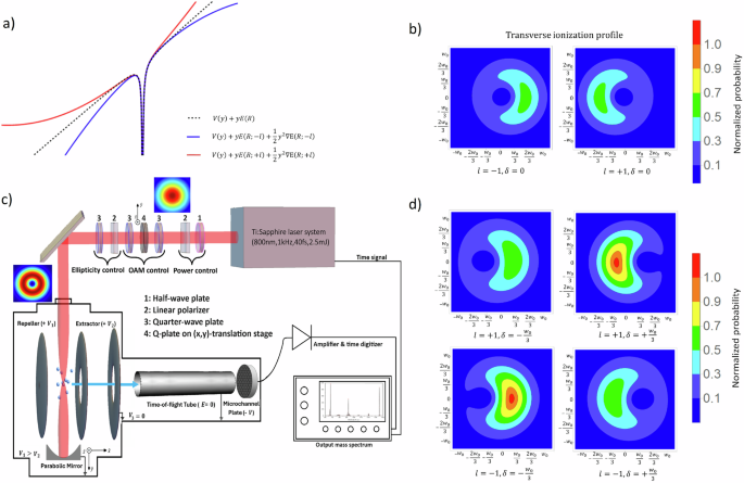
and imaging, some of which are explored in detail later in this article. RESULTS The basic concept of OAM-dependent ionization is illustrated in Fig. 1a by considering the distortion of the

atomic potential caused by the incident light field. For a Gaussian beam, the atomic potential is tipped by the applied electric field (black dotted curve in Fig. 1a), allowing the

electrons to tunnel through the barrier. This non-resonant strong-field ionization is significantly influenced by the peak of the laser field. This conventional picture does not include

higher-order multipole effects. Beyond the dipole approximation, the electric quadrupole term depends on the field gradient ( ∇ _E_). For LG beam, the transverse profile in Cartesian

coordinates is given by $${{{{\bf{E}}}}}_{0,l}^{\pm }(x,y,z)={E}_{0}\frac{{w}_{0}}{w(z)}{\left(\frac{\sqrt{2}}{w(z)}\right)}^{| l| }{\left[\left(x\pm iy\right)\right]}^{| l| }\exp

\left[-\frac{{r}^{2}}{{w}^{2}(z)}\right] \\ \exp \left[ikz-ik\left(\frac{{r}^{2}}{2R(z)}\right)+i(| l|+1)\psi (z)\right]$$ (1) where the handedness of the helical phase is represented by the

± , ∣_l_∣ is the azimuthal index, the radial index is set to zero _p_ = 0, _E_0 is the field amplitude, _w_(_z_) is the beam waist, \(r=\sqrt{{x}^{2}+{y}^{2}}\), _k_ is the wave number,

_R_(_z_) is the radius of curvature, and _ψ_(_z_) is the Gouy phase. Taking a gradient of this field leads to a factor of ± ∣_l_∣ that either enhances or reduces the potential distortion

(blue and red curves in Fig. 1a). Helicity-dependent distortion of atomic potential is purely a phase effect and does not exist in non-OAM beams. To understand the origin of OAM-dependent

ionization, we considered the SFA of tunnel ionization and extended it to include contributions from multipole moments for an asymmetrical LG beam. In the standard SFA model, the transition

amplitude from the ground to the final state, in atomic units, is given by refs. 32,33 $${M}_{fg}=-i {\int}_{-\infty }^{t}\left\langle \right.{\psi }_{V}({t}^{{\prime} })| V({t}^{{\prime}

})| {\psi }_{g}({t}^{{\prime} })\left.\right\rangle d{t}^{{\prime} },$$ (2) where \(V({t}^{{\prime} })\) is the interaction Hamiltonian within dipole approximation, \(| {\psi

}_{g}({t}^{{\prime} })\left.\right\rangle\) is the ground state wavefunction, and \(\left\langle \right.{\psi }_{V}({t}^{{\prime} })|\) is the Gordon-Volkov continuum wavefunction, which is

a plane wave modulated by the laser field. To introduce higher-order multipoles in the interaction Hamiltonian, we Taylor expanded the vector potential to the second order about a point _R_

in the velocity gauge and transformed it to the length gauge to obtain \(\hat{V}({t}^{{\prime} })={r}_{i}{E}_{i}(R,{t}^{{\prime} })+\frac{1}{2}{r}_{i}{r}_{j}\widehat{{\partial

}_{j}{E}_{i}}(R,{t}^{{\prime} })+\frac{1}{2}{L}_{i}{B}_{i}(R,{t}^{{\prime} })\), where _E__i_(_R_, _t_) and _B__i_(_R_, _t_) are the incident electric and magnetic fields of the asymmetrical

LG laser beam (see Supplementary section 6), _r__i_,_j_ is the coordinates of the quadrupole moment i.e. the distance between positive and negative charge in the atom frame, and _R_

represent the coordinates of the laser beam profile. \(\widehat{{\partial }_{j}{E}_{i}}\) represents the field gradient tensor and _L__i_ is the orbital angular momentum of the magnetic

dipole transition moment. The expanded Gordon-Volkov wavefunction that includes the higher order multipoles is therefore given by $${\Psi }_{V}\left(r,t\right)=\frac{1}{{\left(2\pi

\right)}^{3/2}}{e}^{i\left(p+A(R,{t}^{{\prime} })-{\int}_{{t}^{{\prime} }}^{t}\widehat{{\partial }_{R}A}(R,\tau )\left(p+A(R,\tau )\right)d\tau \right)\cdot \, r} \, \\ \times

{e}^{-\frac{i}{2} {\int} _{{t}^{{\prime} }}^{t} {\left(p+A(R,{t}^{{\prime\prime} })- {\int} _{{t}^{{\prime\prime} }}^{t}\widehat{{\partial }_{R}A}(R,\tau )\left(p+A(R,\tau )\right)d\tau

\right)}^{2}d{t}^{{\prime\prime} }},$$ (3) where _A_(_R_, _t_) is the vector potential of the laser field, _p_ is the electron momentum and \(\widehat{{\partial }_{R}A}(R,t)\) is the vector

potential gradient tensor (see Supplementary section 5). Within the dipole approximation, the field gradient tensor term does not exist in the Gordon-Volkov wave function. The full

transition amplitude used to describe the tunnel ionization probability is given by $$M_{fg}= -i\int_{-\infty}^{t}\left[\underbrace{\left\langle{\pi\left(p,t,t^{\prime}\right)}\left\vert

r_{i}\right\vert {\psi_{g}}\right\rangle E_{i}(R,t^{\prime})}_{{{{\rm{E}}}}1}+\underbrace{\frac{1}{2} \left\langle{\pi\left(p,t,t^{\prime}\right)}\left\vert

r_{i}r_{j}\right\vert{\psi_{g}}\right\rangle {\widehat{\partial_{j} E_{i}}}(R,t^{\prime})}_{{{{\rm{E}}}}2} \right. \\

\left.+\underbrace{\frac{1}{2}\left\langle{\pi\left(p,t,t^{\prime}\right)}\left\vert L_{i}\right\vert {\psi_{g}}\right\rangle B_{i}(R,t^{\prime})}_{{{{\rm{M}}}}1}\right] \times

{\exp}\left(\frac{i}{2}\int^{t}_{t^{\prime}}\left(\pi^{2}\left(p,t,t^{\prime\prime}\right)+2I_{p}\right)dt^{\prime\prime}\right)dt^{\prime},$$ (4) where $$\pi \left(p,t,{t}^{{\prime\prime}

}\right)=p+A(R,{t}^{{\prime\prime} })-{\int}_{{t}^{{\prime\prime} }}^{t}\widehat{{\partial }_{R}A}(R,\tau )\left(p+A(R,\tau )\right)d\tau .$$ (5) Equation (4) consists of three terms:

\({M}_{fg}^{{{{\rm{E}}}}1}\), \({M}_{fg}^{{{{\rm{E}}}}2}\), and \({M}_{fg}^{{{{\rm{M}}}}1}\) which are the electric dipole, electric quadrupole, and magnetic dipole transitions,

respectively. The probability of transition is given by $${P}_{fg}=\left| {M}_{fg}^{{{{\rm{E}}}}1}+c{M}_{fg}^{{{{\rm{E}}}}2}+{M}_{fg}^{{{{\rm{M}}}}1} \right|^{2}.$$ (6) The probability

contains a weighting factor _c_ to adjust the relative strength of the electric quadrupole transitions. Both magnetic dipole and electric quadrupole transitions are typically  ~ 10−5 - 10−6

times weaker compared to dipole transitions34, with their strength scaling inversely with the square of the fine structure constant. However, the electric quadrupole moments of atoms are

known to be greatly enhanced by a few orders due to the hyperfine interaction of atomic electrons with the nucleus35,36,37. The weighting factor c was obtained by taking the ratio, _c_ = 

_Q_/_Q__N_, where _Q_ = _Q__N_ + _Q__μ_ + _Q__Q_ is the total quadrupole moment of the atom, _Q__N_ is the nuclear quadrupole moment and _Q__μ_ (Q_Q_) is the induced quadrupole moment due to

the hyperfine interaction between the electron and magnetic dipole (electric quadrupole) of the nucleus. Our model, based on SFA, does not take into account the influence of nucleus on the

energy levels, thereby, ignoring the hyperfine interactions. As a result, higher _c_ − values are required for quantitative analysis. To simulate the transverse ionization probability

profile, we used the ground state 3p-orbital of argon and the electric field represented by the LG beam (Eq. (1), also see Supplementary Section 6), and solved the electric dipole, magnetic

dipole, and electric quadrupole transition matrix elements in momentum space represented by canonical momentum \(\pi (p,t,{t}^{{\prime} })\) with _c_ = 200. For argon 3p state, the c-value

varies within the order of 102-103 for a total atomic angular momentum of _F_ = _I_ ± 1/2 and _F_ = _I_ ± 3/2. The resulting time component of the transition from ground to the continuum was

evaluated using saddle point integration (see Eqs. (28)–(33) in Methods for theory). Figure 1 b shows the transverse ionization probability profile for _l_ = ± 1 at _δ_ = 0. The average

ionization probability is identical for left- and right-helical light. However, a horizontal cut across the beam cross-section reveals an asymmetry in the distribution, with a greater

presence on the left (right) for _l_ = + 1 (_l_ = − 1). Figure 1b suggests that probing the ionization locally would display an asymmetry in angular distribution of electrons akin to that

observed in photoelectron circular dichroism experiments38,39, albeit with linearly polarized helical light beams. However, spatial averaging over the beam cross-section causes the field

gradient term to vanish. So, for symmetric LG beams, the total ion yields are expected to be independent of helicity of light and comparable to a Gaussian beam. The effect of spatial

averaging can be negated by displacing the singularity from the center of the beam to generate asymmetric LG beams. Experimentally, such beams can be produced by translating a phase plate

used to generate OAM beams perpendicular to the incident Gaussian beam (Fig. 1c and Methods section 1.3) or by the coherent superposition of Gaussian and LG beams12. Theoretically, an

asymmetrical LG beam is given by $${{{{\bf{E}}}}}_{0,l}^{\pm }(x,y,z)= {E}_{0}\frac{{w}_{0}}{w(z)}{\left(\frac{\sqrt{2}}{w(z)}\right)}^{| l| }{\left[\left(x\pm i\eta \delta \right)\,\pm

\,i\left(y\,\mp \,i\zeta \delta \right)\right]}^{| l| }\exp \left[-\frac{{r}^{2}}{{w}^{2}(z)}\right]\\ \times \exp \left[ikz-ik\left(\frac{{r}^{2}}{2R(z)}\right)+i(| l|+1)\psi (z)\right]$$

(7) where _δ_ is the displacement of the singularity that can take both negative and positive values and _η_, _ζ_ are used to displace the singularity anywhere in the x-y plane with values

between 0 and 1 (See Supplementary Section 6). In asymmetric LG beams, the field gradient for both handedness at a specific position of the singularity (_δ_-position) are different

(\(\widehat{{\nabla }_{j}{E}_{i}}(+l,\pm \, \delta ) \, \ne \, \widehat{{\nabla }_{j}{E}_{i}}(-l,\pm \delta )\)) and survive spatial averaging. The field gradients amplify the _l_-dependent

distortion of the atomic potential (Fig. 1a), enabling to manipulate the rate of ionization by displacing the phase singularity. Figure 1 d shows transverse profiles of ionization

probabilities for asymmetric LG beams when the singularity is displaced to either side of the center. Compared to symmetric LG beams (Fig. 1b), the asymmetry in the angular distribution of

ionization disappears for asymmetric LG beams. However, the average ionization probability is modulated by changing the handedness of the helicity of light and scales with higher _l_-values.

At _δ_ = − _w_0/3, the average ionization probability is greater for _l_ = − 1 relative to _l_ = + 1. The trend reverses for _δ_ = + _w_0/3, with _l_ = + 1 producing higher ionization

compared to _l_ = − 1. In the absence of the helical phase, synthesized light fields with strong field gradients would not induce strong modulation of ionization. The key advantage of OAM

beams is the handedness of the helical phase that enables to suppress/enhance ionization. While phase singularity remains crucial even in asymmetric LG beams, the field gradients enable to

overcome the effect of spatial averaging, leading to the observation of OAM-dependent ionization yields. To probe OAM-dependent strong-field ionization of atoms and molecules, we measured

the ion yields using time-of-flight mass spectrometer (TOFMS). Figure 1c shows the schematic of the experimental setup. Near-infrared femtosecond laser pulses are focused by a parabolic

mirror inside a differentially pumped vacuum chamber. The ions produced in the interaction region were accelerated towards a field-free drift region and are subsequently detected by

microchannel plates in chevron geometry. The ion signal was then amplified, discriminated, and recorded by a time digitizer to generate a TOF mass spectrum (see Supplementary Fig. S4). A

_q_-plate was used to convert the incident Gaussian beam to an OAM beam via spin-orbit coupling. Optical components such as waveplates and polarizers were used to control the incident power

and laser polarization. Translating the _q_-plate with respect to the incident beam generated asymmetric OAM beams in which the phase singularity (and hence the null intensity region) is

displaced within the focal spot (See Methods for experimental details). Figure 2 shows the experimental results of the ionization of argon atom for _l_ = ± 1 (a, b) and _l_ = ± 3 (c, d) as a

function of the position of the singularity, _δ_. For a symmetric OAM beam (_δ_ = 0), the singly charged ion yields are identical for left- and right-handed helical light (Fig. 2a, c). When

the singularity is displaced to +_δ_, the ion yields for  + _l_ (black curve) increase and reach a maximum. When the handedness is changed to  − _l_ (red curve), the ion yields are maximum

at  − _δ_. Therefore, the _δ_-dependence of the ion yields for  − _l_ mirrors that of  + _l_ about _δ_ = 0. At higher _l_-values, the ratio of the maximum ion yields at _δ_ ≠ 0 to the ion

yields at _δ_ = 0 increase for a specific handedness of the helical light (Fig. 2a, c). The increase in the ion yields for an asymmetric OAM beam arises from the growing peak field strength

and the difference in the field gradient as the singularity is displaced (refer to Fig. 1). However, at large _δ_ positions, the ion yields decrease because of the diminishing peak field

strength as the beam profile starts resembling a Gaussian-like beam (see Supplementary Fig. S12). At a specific _δ_-position, the difference in ionization between the left- and right-helical

light persists up to saturation intensity (see Supplementary Fig. S6). The degree of control achieved using asymmetric OAM beams is significantly higher, by two orders of magnitude, when

compared to conventional pulse shaping techniques27,28,29 that typically operate mostly within dipole approximation. Selective ionization with linearly polarized asymmetric helical light of

opposite handedness leads to dichroism - a property typically observed in chiral molecules with broken symmetry. In our case, the interplay between the helicity of light and the broken

symmetry, introduced by the _δ_-parameter, results in a differential response of argon. Figure 2b, d illustrate differential ionization in argon, for _l_ = 1, 3, respectively, when subjected

to linearly polarized helical light of opposite handedness. This difference, denoted as Δ_Y_(_l_) = _Y_( + _l_, _s_ = 0) − _Y_( − _l_, _s_ = 0), is known as Helical Dichroism (HD) and

exhibits a characteristic sinusoidal shape. This phenomenon is akin to the recently observed nonlinear absorption of helical light in chiral and achiral liquids and solids17,18. As _δ_

increases, Δ_Y_ will rise to a maximum around _δ_ = ± _w_0/3 for _l_ = 1 and decrease at the large _δ_-position. This is because as the position of the singularity approaches the periphery

of the beam’s cross-section it starts to resemble a symmetric Gaussian beam profile. Notably, in Fig. 2d the difference in the yields Δ_Y_(_l_ = 3) is maximum at a larger _δ_-position and

exhibits an intriguing feature around _δ_ = 0, resembling an inflection point. This behavior is affected by the incident intensity and arises because the size of the singularity is greater

for _l_ = 3 relative to _l_ = 1, necessitating a larger displacement to observe an appreciable increase in the ion yield. The phenomenon of OAM-dependent ionization is not confined to atoms

but also extends to molecules. Figure 3a, c show how the singly charged ion yields vary with the singularity position (_δ_) for _l_ = ± 1 in two molecules: R(+)-limonene (chiral molecule)

and acetone (achiral molecule). In chiral systems, the two enantiomers that are non-superimposable mirror images, are discernible only when they interact with another chiral system. A

typical optical probe exploits the broken symmetry of the handedness of circularly polarized light resulting in differential absorption of left- and right-handed polarizations, leading to

circular dichroism. However, enhanced chiral sensitivity was achieved recently in chiral liquids and solids17,18 by transferring this broken symmetry to the helical phase of the light rather

than its polarization. In achiral systems, the conventional understanding is that dichroism does not occur due to the presence of _S__n_ symmetry. However, achiral liquids and solids

exhibited dichroism when irradiated with asymmetric OAM beams, where the symmetry is broken spatially in the beam profile and the phase of light. This raises the question of whether helical

dichroism can also be observed in the gas phase. For both molecules, the _δ_-dependence of ion yields for  − _l_ mirrors that of the  + _l_ about _δ_ = 0, similar to argon. The ion yields

are identical at _δ_ = 0, and this mirroring behavior was also present for the ionization of limonene with higher-order _l_-values (See Supplementary Fig. S7a). Unlike argon, both molecules

display an asymmetric double bump structure for a specific handedness of helical light. This is likely due to differences in their ionization potentials (8.5 eV for limonene, 9.7 eV for

acetone, and 15.6 eV for argon). The double bump feature is influenced by the laser intensity and the strength of the E1E2 coupling term (see Supplementary Fig. S1a, b) and becomes more

pronounced with increasing intensity approaching saturation. Strong field ionization with OAM beams is a consequence of the interplay between peak field strength and field gradients. The

latter gives rise to helicity-dependent ionization, while the former determines the overall ionization rate. At laser intensities approaching saturation, the peak field strength dominates

the gradient contribution, leading to higher ionization rates but reduced differences in ionization between the left- and right-handed helical light (see Supplementary Fig. S6 insets) due to

ground state depletion. At intensities well below saturation, the field gradient contribution dominates and has a greater impact on the helicity-dependent ionization rate. As a result, one

handedness of helical light can completely suppress ionization, eliminating the asymmetrical double bump feature. In molecules, the experimental intensities used (8–9  × 1013 W/cm2) were

closer to their saturation intensities compared to argon. Figure 3 b, d show HD in R(+)-limonene (see Supplementary Fig. S5 for S(−)-limonene) and in acetone, respectively, when subjected to

linearly polarized helical light of opposite handedness, exhibiting the same sinusoidal shape as shown in Fig. 2b. Similar results were obtained when the laser polarization was changed from

linear to circular (see Supplementary Fig. S8). For a specific _δ_ position, the ion yields are predominant for one handedness irrespective of the ellipticity, _ε_, of light (see

Supplementary Figs. S9, S10). For higher order _l_-value, limonene exhibits a similar inflection point as argon (Fig. 2d), as shown in Fig. S7b in the Supplementary. For a specific

enantiomer, left- and right-handed helical light produced different ion yields. However, for a specific helicity of light, the ion yields remained similar for the two enantiomers (see

Supplementary Fig. S5) within the experimental errors, in contrast to the enhanced chiral sensitivity observed in liquids and solids17,18. For the intensities used in the experiments, tunnel

ionization is predominant where the electron transitions mostly from the ground state to continuum and does not involve the chiral-sensitive excited states. Therefore, the ionization rates

are expected to be similar for both enantiomers, albeit in different directions. So, probing the electron angular distributions would provide more chiral sensitivity than the total ion

yields. To simulate the experimental results (Figs. 2, 3), we plotted the electric transition probability (Eq. (6)) integrated over the beam cross-section, given by

\({\overline{P}}_{fg}={\int}_{-{w}_{0}}^{{w}_{0}}| {M}_{fg}^{{{{\rm{E}}}}1}+c{M}_{fg}^{{{{\rm{E}}}}2}+{M}_{fg}^{{{{\rm{M}}}}1}{| }^{2}dR\). The only coupling term that contains _l_ −

dependence is the E1E2 term due to the presence of the field gradient. The mixed coupling term E1M1 is responsible for circular dichroism and does not contribute to the differential signal

for linearly polarized light. Figure 4 a depicts the differential ionization probability between left- and right-helical light as a function of displacement of the singularity for _l_ = ± 1

and  ± 3. These probabilities, obtained at _c_ = 1, mirror the experimental results shown in Figs. 2b, d and 3b, d. For higher _l_ − values, the null intensity region is larger, leading to

stronger field gradients and higher peak field strengths. Consequently, differential ionization is enhanced but exhibits an inflection point around _δ_ = 0, accompanied by a change in the

slope, as larger displacements of the singularity are required to significantly alter the ion yield. This inflection point becomes more pronounced at higher laser intensities. While the

behavior of differential ionization with the asymmetry parameter _δ_ is independent of the _c_ − value, visualization and comparison of ionization probabilities with experimental ion yields

from Fig. 2a, c necessitate amplifying quadrupole transitions. Figure 4b illustrates the dependence of ionization probability on the displacement of the singularity for different _l_ − 

values using _c_ = 200, chosen to show the double bump feature that also depends on the laser intensity (Supplementary Fig. S1a). The ionization as a function of _δ_ − position exhibits an

asymmetric double bump structure. This asymmetry increases with _l_ − value, laser intensity and _c_ − value (see Supplementary Fig. S1a, b). It vanishes at low intensities and becomes

prominent at higher intensities until the ground state is depleted. Moreover, the symmetry of the double bump structure is affected by the angle through which the singularity is displaced

across the center (see Supplementary Fig. S2). A quantitative comparison of the ionization probability with the experimental results of Fig. 2a, c could be obtained for _c_ = 400 or higher

(see Supplementary Fig. S1b). This c-value is within the range of two to three orders of magnitude of the quadrupole moment enhancement due to the hyperfine interactions. DISCUSSION The

subtle differences in the distortion of the atomic potential shown in Fig. 1, induced by left- and right-handed OAM beams, give rise to intriguing phenomena in strong-field physics. They

have the potential to imprint characteristic features on the angular distribution of the ionized electron with a preferred directionality by changing either the handedness of helical light

or the sign of _δ_-position. When extended to chiral molecules, the asymmetry in the molecular potential could increase/decrease the photoelectron emission along a particular direction. This

can lead to efficient chiral discrimination, analogous to photoelectron circular dichroism, and be further enhanced through the utilization of higher _l_-values. Moreover, the

directionality of the ejected electron can be controlled by angular rotation of the singularity in the transverse plane of the laser focus. This capability provides an additional control

parameter to manipulate the molecular potential manifold and, therefore, the reaction dynamics. Additionally, the transverse spreading of the ionized electron wavepacket can be influenced,

thereby affecting recollision dynamics (see Supplementary Fig. S11). The peak field strength varies across the beam profile when the singularity is displaced in an OAM beam. It rises with

_δ_ and eventually reaches a maximum. As _δ_ increases further, approaching the edge of the beam cross-section, the peak field strength decreases as the beam profile starts resembling that

of a Gaussian beam. This variation in the peak field strength has a direct impact on the ponderomotive energy of the free electron, as depicted in Fig. 5a. At higher _l_-values, the null

intensity region expands, and the field gradient intensifies. Consequently, the ponderomotive energy increases with _l_-value and reaches a maximum at smaller _δ_ values. Similar

enhancements in ponderomotive energy are feasible with synthesized light beams that do not have a helical phase. Such non-OAM beams can be produced by coherent superposition of

Hermite-Gaussian beams with an intensity profile that resembles that of an asymmetric LG beam. However, the use of asymmetric LG beams offers a convenient knob to control ponderomotive

effects instead of coherent superposition of multiple beams. While the increase in ponderomotive energy is mainly due to the intensity variation, the ionization modulation observed with OAM

beams (Figs. 2–4) results from the interplay between the helical phase and field gradients. This becomes evident when the effects of the helical phase and field gradient are isolated by

simulating the ionization probability for non-OAM structured light beams (see Supplementary Fig. S3). The probability exhibits a symmetrical double bump behavior due to the lack of OAM, in

contrast to the asymmetry seen in Fig. 4b. Therefore, the helical phase can impact associated phenomena in strong-field physics. In asymmetric LG beams, the multipole contributions couple

from the carrier phase into the envelope, resulting in strong intensity modulations on the order of a wavelength. The carrier phase varies on a much shorter length scale than the electric

field envelope. As such, the resulting multipole effects rooted in the carrier phase affect the ponderomotive force much stronger than the modulation of the pulse envelope alone. This is

unique to OAM beams and is hard to achieve by methods that manipulate the envelope alone. So, phase singularity and field gradients are intertwined, as highlighted in the transition

amplitude describing the tunnel ionization probability Eq. (4). It consists of two contributions: the electric quadrupole and magnetic dipole both in the pre-exponent and in the classical

action via the vector potential gradient. The electric quadrupole (E1E2) in the pre-exponent affects only ionization and survives averaging for asymmetric beams. The non-dipole terms of the

classical action in the exponential changes the electron trajectory - not important for ionization but for high harmonic generation (HHG) and acceleration. The tunability of ponderomotive

energy with asymmetric OAM beams significantly impacts HHG, a critical process in attosecond science. Transitioning from a Gaussian beam to an asymmetric OAM beam, at an intensity of 1014

W/cm2, results in a threefold increase in ponderomotive energy for _l_ = 9. This translates to extending the cut-off harmonics (3.17 U_p_) by the same amount without the need for a laser

operating at longer wavelengths. For example, an 800 nm asymmetric OAM beam would generate the same cut-off harmonics as a laser operating at 1500 nm with a Gaussian profile. Moreover, the

drift energy of the electron (Up to 2U_p_), which is proportional to the ponderomotive energy, can be regulated by displacing the singularity within the transverse plane of the laser focus.

However, the temporal electron dynamics in the laser field, _vis-à-vis_ ionization and recollision times, remains the same for both Gaussian and OAM beams as shown in Fig. 5c. At a specific

position of the singularity (_δ_ = _w_0/3), the kinetic energy of the recolliding electron increases with _l_-value but its temporal dynamics is not influenced by the _l_-value or asymmetry

parameter _δ_. The controlled generation of electron wavepackets with asymmetric OAM beams also facilitates the probe of molecular dynamics by taking snapshots of conformational

transformations. This is possible either by scattering of the electron wavepacket from its parent molecular ion (i) elastically, leading to a diffraction pattern, or (ii) inelastically,

leading to multiple ionization and fragmentation from which changes to bond length and angles could be extracted. The ability to increase the ponderomotive energy of the electron with OAM

beams enhances the spatial resolution in such studies. Figure 5 b illustrates the variation of the average ponderomotive force in the focal plane as a function of the displacement of the

singularity, _δ_, for different _l_-values. This force was obtained by integrating over the cross-section of the laser beam at the focus and depends on the gradient of the intensity. For a

Gaussian beam, the average ponderomotive force is zero, represented by a circle. The behavior is similar for symmetric OAM beams. However, when the singularity is displaced, the

ponderomotive force exhibits local maxima and minima that increase with the _l_-value. The position of local maxima and minima in the ponderomotive force aligns with specific _δ_ values

where differential ionization exhibits maximum magnitude. In plasma physics, a factor of forty enhancement in ponderomotive force with asymmetric OAM beams facilitates the acceleration of

charged particles to higher energies compared to Gaussian beams. This method serves as an alternate to the use of temporally asymmetric laser pulses to manipulate the characteristics of

accelerated charged particles40,41,42. In addition, at a given intensity, _l_-dependent ionization of matter also enables to precisely control plasma density by an order of magnitude

compared to a Gaussian beam. This could potentially be harnessed, for example, to manipulate laser filamentation and enhance its application in electromagnetic waveguiding and remote sensing

of atmospheric molecules for accurate environmental monitoring. Another application of asymmetric helical light pulses is towards super-resolution imaging due to their ability to localize

and control light intensity to sub-wavelength dimensions. Figure 6a–d show the transverse intensity profiles for Gaussian and asymmetric LG beams in which the beam waist is fixed to the

wavelength of light. As the OAM value increases, the light intensity is redistributed to a smaller bean-shaped area, and the peak intensity increases. Any nonlinear process, such as the

multiphoton excitation of a fluorophore, exhibits a threshold intensity above which it emits radiation. By setting the threshold intensity at 90% we extracted the dimensions of the localized

hot-spot and plotted it as a function of the OAM value, as shown in Fig. 6e. The size of the hot-spot is reduced by increasing the _l_-value with the x-dimension smaller than the

y-dimension by a factor of two. Such localization can be combined with the ability to manipulate photoexcitation by changing the _δ_-position and helicity (as shown in Fig. 1b for

ionization) to enhance the spatial resolution by a factor of 2–3 times the diffraction limit. This is a much simpler technique to create a localized hot-spot but is mostly restricted to

one-dimension. This is in contrast to complicated methods such as hot-spot localization by the superposition of several coherent beams43 or stimulated emission depletion involving two color

coherent beams that require specially designed fluorophores that can be excited and deexcited44,45. In conclusion, we demonstrated _l_-dependent ionization of atoms and molecules that can be

precisely controlled by manipulating the phase singularity within the OAM beam. We extended strong-field tunnel ionization beyond the dipole approximation to simulate the ionization of

atoms. Our study provides valuable insight into the intricate mechanisms underlying strong-field physics. As discussed above, OAM beams provide an additional tool to manipulate extreme

nonlinear processes that drive a spectrum of research domains. In spectroscopy, it allows us to probe conformational changes in molecules with enhanced spatial resolution. In attosecond

science, it enables efficient generation of higher-order harmonics at shorter wavelengths. In plasma physics, it facilitates the efficient production of higher-energy charged particles.

Additionally, by modifying the plasma density, laser filamentation can be effectively employed for remote sensing applications. In imaging, aysmmetric OAM beams enable us to localize

photoexcitation of flourophores to achieve sub-wavelength spatial resolution. METHOD IONIZATION MEASUREMENTS Experiments were conducted by focusing near-infrared femtosecond laser pulses

with a parabolic mirror (focal length 5 cm) in the interaction region of a TOFMS housed inside a differentially pumped vacuum chamber. A Ti:Sapphire laser system (Spitfire, Spectra-Physics)

operating at _λ_ = 800 nm and a repetition rate of 1 KHz produced  ~40 fs pulses with a maximum pulse energy of  ~2.5 mJ. A combination of a half-wave plate and a polarizer were used to

control the pulse energy. The pulse duration was continuously monitored by a single-shot autocorrelator. A fast photodiode was used to continuously monitor the laser pulse energy incident on

a 3 mm thick quartz window on the vacuum chamber. The ions produced in the interaction region of TOFMS, operated in Wiley-McLaren geometry, travel through a field-free region of 30 cm after

acceleration and are detected by a microchannel plate in chevron geometry. The signal is then amplified, discriminated, and recorded by a time digitizer to generate a TOF mass spectrum. The

voltage on the microchannel plates was set at −4900 V. The voltages on the repeller and extractor plates of the mass spectrometer were +2000 V and +1000 V, respectively. A precision leak

valve was used to introduce atoms and molecules in gas phase. The pressure inside the vacuum chamber was maintained at  ~10−6 Torr. Organic compounds like limonene and acetone had sufficient

vapor pressure, at room temperature, to be introduced as a gas. They were subjected to freeze-and-thaw cycles to minimize contamination of the interaction region. To minimize number density

fluctuations, the chemicals in the glass vial were immersed in a temperature bath at 22 °C and the gas line along with the leak valve were maintained at a positive temperature gradient. The

S(−)-limonene and R(+)-limonene were sourced from Sigma Aldrich with a purity of 96% and 97%, respectively. Measurements in limonene and acetone were performed at an intensity of 8–9 × 1013

W/cm2, below the measured saturation intensities of  ~12−13 × 1013 W/cm2. Measurements in argon were performed at an intensity of 9−15 × 1013 W/cm2. The differential ionization curves were

obtained by displacing the position of singularity in the cross-section of the OAM beam. A pair of mass spectra, measured for 100,000 laser shots, were recorded for each handedness of the

incident helical light. Fluctuations of the ion yields and error bars related to the differential ionization signal were computed based on repeated measurements under similar conditions.

CALIBRATION OF MASS SPECTROMETER, LASER INTENSITY AND ELLIPTICITY Mass calibration was achieved using Xenon atoms. Mass resolution of the spectrometer (full width at half maximum) was 550 at

an _m_/_z_ (mass-to-charge ratio) of 132. Laser intensity was calibrated by measuring the saturation intensity of argon. This was achieved by plotting Ar+ yields as a function of pulse

energy. The intercept on the energy axis of the semi-log plot corresponds to the theoretical saturation intensity of  ~2.5 × 1014 W/cm2. The extracted focal spot size in the interaction

region was 3  ± 0.2 _μ_m, in agreement with previous measurements. A quarter-wave plate (QWP) was used to change the ellipticity, _ϵ_, of the polarized helical light beam. It was calibrated

by measuring the ellipticity dependence of doubly charged argon. We obtained _ϵ_ = 0.05 for linear polarization and _ϵ_ = ± 0.96 for circular polarization, with an uncertainty of  ± 0.02.

The ellipticity was varied in steps of 0.04 around linear polarization and in steps of 0.08 beyond _ϵ_ = 0.2. GENERATION OF OAM BEAMS AND DISPLACEMENT OF SINGULARITY A QWP on a motorized

rotation stage (with a  ± 0.005° resolution) was used to generate circularly polarization light that was incident on a birefringent liquid-crystal-based phase plate called a q-plate.

Circularly polarized Gaussian beam propagating through the q-plate with a topological charge q, acquires an OAM defined by _l_ = ± 2_q_, with a phase singularity and hence a null intensity

region at the center of the beam, known as an optical vortex. The handedness of the incident circular polarization determines the direction of rotation of the wavefront structure _i_. _e_.

the handedness of the helical light. A second QWP was used to generate linearly polarized OAM beams. The conversion efficiencies of the q-plates were  ~86 ± 2% for _l_ = 1 and  ~88 ± 2% for

_l_ = 3. The singularity in the OAM beam was displaced by translating the q-plate across the incident beam, whose diameter was 12 mm. The q-plate, mounted on a motorized xy-translation stage

with a precision of 10_μ_m, was displaced in steps of 500  ± 10_μ_m. When focused by the parabolic mirror, this translated to a displacement step size of 330  ± 60 nm in the interaction

region with respect to the center of the beam. The calibration was achieved by measuring the total translation required to displace the singularity to the periphery of the defocused beam and

comparing it to the measured spot size of _w_0 = 3  ± 0.2 _μ_m. An alternate method of displacing the singularity is by the coherent superposition of OAM beam with a tunable amount of a

linearly polarized Gaussian beam12. The central singularity either shifts or unfolds into multiple singularities, depending on the topological charge of the q-plate. This shift can be

precisely controlled by adjusting the external field applied to the q-plate. This action varies the optical retardation, thereby detuning the strength of the spin-to-orbital angular momentum

coupling of light. A fraction of the input Gaussian beam co-propagates with a partially converted OAM beam. THEORY Tunnel ionization of an atom is often described using SFA, where the laser

field strength is comparable to the Coulomb field of an atom. It is predominant when the laser frequency is slower than the frequency of electron tunneling through the barrier. SFA assumes

that only the ground state and the continuum are involved in the dynamics and that the intermediate states and ground state depletion are neglected. Ionization probability can be obtained

from the transition amplitude defined as a projection of the final state _ψ__f_(_t_) to a fully evolved ground state at large times32,33, given by \({M}_{fg}={\lim }_{t\to \infty }\langle

{\psi }_{f}(t)| \Psi (r,t)\rangle\), where _Ψ_(_r_, _t_) is the total wave function of time-evolved ground state, _ψ__g_, when the laser field is turned on. _Ψ_(_r_, _t_) is a solution of

the time-dependent Schrodinger equation and is solved using the Green function \(\hat{G}(t,{t}^{{\prime} })=-i\Theta (t-{t}^{{\prime} })\hat{U}(t,{t}^{{\prime} })\)32,33 where \(\Theta

(t-{t}^{{\prime} })\) is the Heaviside step function and \(\hat{U}(t,{t}^{{\prime} })\) is a unitary time operator. By using the orthogonality of the wavefunctions, the Born approximation

where the perturbation acts only on the ground state, and approximating the final state as a Volkov wavefunction; \(\left\langle \right.{\psi }_{f}(t)| \hat{U}(t,{t}^{{\prime} })\to

\left\langle \right.{\psi }_{V}({t}^{{\prime} })|\) we obtain the general SFA tunneling transition amplitude from the ground state to the continuum given by $${M}_{fg}=-i {\int}_{-\infty

}^{\infty }d{t}^{{\prime} }\left\langle \right.{\psi }_{V}({t}^{{\prime} })| \hat{V}({t}^{{\prime} })| {\psi }_{g}({t}^{{\prime} })\left.\right\rangle$$ (8) In standard SFA, only the

electric dipole moment is considered in the interaction Hamiltonian and in the Volkov wavefunction. In principle, the transition amplitude can be expressed either in velocity or length

gauges. Conversion from one gauge to the other can be achieved by using the generating function \(\chi (r,R,t)=\int_{0}^{1}\overrightarrow{r} \, \cdot \, \overrightarrow{A}(R+\lambda

r,t)d\lambda\) and its resulting unitary operator _e_−_i__χ_(_r_, _R_, _t_)46. In the velocity gauge, the ground state wavefunction is given by \(| {\tilde{\psi

}}_{g}(t)\left.\right\rangle={e}^{-i\chi (r,R,t)}| {\psi }_{g}(t)\left.\right\rangle\) and the Hamiltonian is given by \(\hat{H}(t)=\frac{1}{2}{\left(-i\overrightarrow{\nabla

}+\overrightarrow{A}({r}^{{\prime} },t)\right)}^{2}\) where \(| {\psi }_{g}(t)\left.\right\rangle\) is the ground state wavefunction in length gauge, \(i\overrightarrow{\nabla }\) is the

momentum operator and \(\overrightarrow{A}({r}^{{\prime} },t)\) is the vector potential. We used the length gauge to derive the transition amplitude. To introduce higher order multipoles in

the interaction Hamiltonian, we * 1. (i) Taylor expanded the vector potential to the second order about a point _R_ in the interaction Hamiltonian as, \(\overrightarrow{A}({r}^{{\prime}

},t)\approx \overrightarrow{A}(R,t)+{\overrightarrow{r}}^{{\mathsf{T}}}\widehat{\partial A}\left(R,t\right)...\), and in the generating function as, \(A(R+\lambda r,t)=A(R,t)+\lambda

{\overrightarrow{r}}^{{\mathsf{T}}}\widehat{\partial A}(R,t)\), where \({\overrightarrow{r}}^{{\mathsf{T}}}\) is the transpose of position vector. * 2. (ii) Applied the unitary

transformation operator _e_−_i__χ_(_r_, _R_, _t_) to explicitly express the existence of electric quadrupole and magnetic dipole in length gauge resulting in the non-dipole interaction

Hamiltonian \(\hat{V}({t}^{{\prime} })={r}_{i}{E}_{i}(R,{t}^{{\prime} })+\frac{1}{2}{r}_{i}{r}_{j}\widehat{{\partial }_{j}{E}_{i}}(R,{t}^{{\prime}

})+\frac{1}{2}{L}_{i}{B}_{i}(R,{t}^{{\prime} })\), where _E__i_(_R_, _t_) and _B__i_(_R_, _t_) are the incident electric and magnetic fields, respectively, of the asymmetrical

Laguerre-Gaussian laser beam (see Supplementary section 6), _r__i_,_j_ is the distance between positive and negative charge in the atomic frame and _R_ represent the coordinates of the laser

beam profile. \(\widehat{{\partial }_{j}{E}_{i}}\) represents the field gradient, and _L__i_ is the orbital angular momentum of the magnetic dipole transition moment. Lastly, we expanded

the Volkov wavefunction to include the higher order multipoles to \(O(\widehat{\partial A})\) and converted it from velocity to length gauge using the first order transformation,

\({e}^{-i\chi \left(r,R,t\right)} \sim {e}^{-iA(R,t) \, \cdot \, r}\) to obtain Eq. (3) of the main text (see Supplementary Section 5). The non-dipole free-electron wavefunction shown in Eq.

(3) can be expressed in terms of time propagator, \({\hat{U}}_{V}(t,{t}^{{\prime} })\), and a plane wave with a momentum \(\pi \left(p,t,{t}^{{\prime} }\right)\) $${\Psi

}_{V}\left(r,t\right)=\frac{{\hat{U}}_{V}(t,{t}^{{\prime} })}{{\left(2\pi \right)}^{3/2}}{e}^{i\pi \left(p,t,{t}^{{\prime} }\right) \, \cdot \, r}={\hat{U}}_{V}(t,{t}^{{\prime} })| \pi

\left(p,t,{t}^{{\prime} }\right)\left.\right\rangle$$ (9) where $$\pi \left(p,t,{t}^{{\prime} }\right)= \left(p+A(R,{t}^{{\prime} })- {\int}_{{t}^{{\prime} }}^{t}\widehat{{\partial

}_{R}A}(R,\tau )\left[p+A(R,\tau )\right]d\tau \right);\quad \\ {\hat{U}}_{V}(t,{t}^{{\prime} })={e}^{-\frac{i}{2} {\int} _{{t}^{{\prime} }}^{t}{\left(p+A(R,{t}^{{\prime\prime} })- {\int}

_{{t}^{{\prime\prime} }}^{t}\widehat{{\partial }_{R}A}(R,\tau )\left[p+A(R,\tau )\right]d\tau \right)}^{2}d{t}^{{\prime\prime} }}$$ Therefore, the length gauge ground state tunneling

transition amplitude up to \(O(\widehat{\partial A})\) becomes $${M}_{fg} =-i {\int} _{-\infty }^{t}d{t}^{{\prime} }\left\langle \right.\pi \left(p,t,{t}^{{\prime} }\right)|

{\hat{U}}_{V}(t,{t}^{{\prime} })V({t}^{{\prime} })| {\psi }_{g}({t}^{{\prime} })\left.\right\rangle \\ =-i {\int}_{-\infty }^{t}d{t}^{{\prime} }\left\langle \right.\pi

\left(p,t,{t}^{{\prime} }\right)| V({t}^{{\prime} })| {\psi }_{g}\left.\right\rangle {e}^{iS\left(p,t,{t}^{{\prime} }\right)}$$ The full transition amplitude describing the tunnel ionization

probability for an asymmetric Laguerre-Gaussian beam, shown in Equation (4) of the main text, can be obtained from $${M}_{fg}= -i {\int}_{-\infty }^{t}d{t}^{{\prime} }\left\langle

\right.\pi \left(p,t,{t}^{{\prime} }\right)| {r}_{i}{E}_{i}(R,{t}^{{\prime} })+\frac{1}{2}{r}_{i}{r}_{j}\widehat{{\partial }_{j}{E}_{i}}(R,{t}^{{\prime} }) \\

+\frac{1}{2}{L}_{i}{B}_{i}(R,{t}^{{\prime} })| {\psi }_{g}\left.\right\rangle {e}^{iS\left(p,t,{t}^{{\prime} }\right)}$$ (10) where $$S\left(p,t,{t}^{{\prime} }\right)=\frac{1}{2} {\int}

_{{t}^{{\prime} }}^{t}\left[{\left(p+A({t}^{{\prime\prime} })- {\int} _{{t}^{{\prime\prime} }}^{t}\widehat{{\partial }_{R}A}\left(p+A(\tau )\right)d\tau

\right)}^{2}+2{I}_{p}\right]d{t}^{{\prime\prime} }$$ (11) To calculate the electric dipole, magnetic dipole, and electric quadrupole moment, we consider the ground state wave function of

argon to be a 3p-orbital given by \(| {\psi }_{g}\left(r\right)\left.\right\rangle={R}_{nl}(r){Y}_{lm}(\theta,\phi )=| nlm\left.\right\rangle\), where _n_, _l_, _m_ are principal, orbital,

and spin quantum numbers. These transition moments are expressed in the momentum space by applying the position operator on the momentum state to obtain $${{{\rm{E}}}}1 =\left\langle

\right.\pi \left(p,t,{t}^{{\prime} }\right)| {r}_{i}| {\psi }_{g}\left(r,{t}^{{\prime} }\right)\left.\right\rangle {E}_{i}\left(R,{t}^{{\prime} }\right)=i{\partial }_{i}| {\psi

}_{g}({{{{\boldsymbol{\pi }}}}}_{{{{\bf{p}}}}})\left.\right\rangle {E}_{i}\left(R,{t}^{{\prime} }\right)\\ {{{\rm{E}}}}2 =\frac{1}{2}\left\langle \right.\pi \left(p,t,{t}^{{\prime} }\right)|

{r}_{i}{r}_{j}| {\psi }_{g}\left(r,{t}^{{\prime} }\right)\left.\right\rangle \widehat{{\partial }_{j}{E}_{i}}(R,{t}^{{\prime} })=-\frac{1}{2}{\partial }_{i}{\partial }_{j}| {\psi

}_{g}({{{{\boldsymbol{\pi }}}}}_{{{{\bf{p}}}}})\left.\right\rangle \widehat{{\partial }_{j}{E}_{i}}(R,{t}^{{\prime} })\\ {{{\rm{M}}}}1 =\frac{1}{2}\left\langle \right.\pi

\left(p,t,{t}^{{\prime} }\right)| {L}_{i}| {\psi }_{g}\left(r,{t}^{{\prime} }\right)\left.\right\rangle {B}_{i}\left(R,{t}^{{\prime} }\right) \\

=\frac{1}{4}\left(\begin{array}{c}\sqrt{l(l+1)-m(m+1)}| {\psi }_{g(m+1)}({{{{\boldsymbol{\pi }}}}}_{{{{\bf{p}}}}})\left.\right\rangle+\sqrt{l(l+1)-m(m-1)}| {\psi

}_{g(m-1)}({{{{\boldsymbol{\pi }}}}}_{{{{\bf{p}}}}})\left.\right\rangle \\ -i\sqrt{l(l+1)-m(m+1)}| {\psi }_{g(m+1)}({{{{\boldsymbol{\pi

}}}}}_{{{{\bf{p}}}}})\left.\right\rangle+i\sqrt{l(l+1)-m(m-1)}| {\psi }_{g(m-1)}({{{{\boldsymbol{\pi }}}}}_{{{{\bf{p}}}}})\left.\right\rangle \\ m| {\psi }_{g}({{{{\boldsymbol{\pi

}}}}}_{{{{\bf{p}}}}})\left.\right\rangle \end{array}\right) {B}_{i}\left(R,{t}^{{\prime} }\right)$$ (12) where the momentum wavefunction is defined as \(| {\psi }_{g}({{{{\boldsymbol{\pi

}}}}}_{{{{\bf{p}}}}})\left.\right\rangle=\langle \pi \left(p,t,{t}^{{\prime} }\right)| {\psi }_{g}\left(r,{t}^{{\prime} }\right)\rangle\) and \(| {\psi }_{g(m\pm 1)}({{{{\boldsymbol{\pi

}}}}}_{{{{\bf{p}}}}})\left.\right\rangle=\langle \pi \left(p,t,{t}^{{\prime} }\right)| nl(m\pm 1)\rangle\). The angular momentum operator is expressed in terms of the raising and lowering

operators \(({L}_{x}=\frac{1}{2}({L}_{+}+{L}_{-}),{L}_{y}=\frac{1}{2i}({L}_{+}-{L}_{-}),{L}_{z})\) and its definition on the spherical harmonics \({L}_{\pm }|

nlm\left.\right\rangle=\sqrt{l(l+1)-m(m\pm 1)}| nl(m\pm 1)\left.\right\rangle\). The momentum wavefunction was obtained by Fourier transforming the spatial radial wavefunction for

hydrogen-like atoms47. $$ FT[{R}_{nl}(r)]={F}_{nl}(p)={\left[\frac{2}{\pi }\frac{(n-l-1)!}{(n+1)!}\right]}^{(1/2)} \\

{n}^{2}{2}^{2(l+1)}l!\frac{{n}^{l}{p}^{l}}{{({n}^{2}{p}^{2}+1)}^{l+2}}{C}_{n-l-1}^{l+1}\left(\frac{{n}^{2}{p}^{2}-1}{{n}^{2}{p}^{2}+1}\right)$$ (13) where \({C}_{n-l-1}^{l+1}\) is the

Gegenbauer polynomial. Therefore, the ground state wave function for argon (3p orbital, _n_ = 3, _l_ = 1, _m_ = 0, ± 1) in momentum space is given by $$\left\vert{\psi_{g(m=\pm

1)}({{{\mathbf{\pi}}}}_{{{{\mathbf{p}}}}})}\right\rangle

=\underbrace{\frac{500}{\sqrt{\pi}}{{{\mathbf{\pi}}}}_{{{{\mathbf{p}}}}}\frac{(9{{{\mathbf{\pi}}}}_{{{{\mathbf{p}}}}}^{2}-1)}{(9{{{\mathbf{\pi}}}}_{{{{\mathbf{p}}}}}^{2}+1)^{4}}}_{F_{3,1}({{{\mathbf{\pi}}}}_{{{{\mathbf{p}}}}})}\underbrace{\left[\mp\sqrt{\frac{3}{8\pi}}({{{\mathbf{\pi}}}}_{p_x}\pm

i{{{\mathbf{\pi}}}}_{p_y})\frac{1}{{{{\mathbf{\pi}}}}_{{{{\mathbf{p}}}}}}\right]}_{Y_{1,\pm 1}(\theta,\phi)} \\ =\mp\frac{34}{81\pi}({{{\mathbf{\pi}}}}_{p_x}\pm

i{{{\mathbf{\pi}}}}_{p_y})\frac{({{{\mathbf{\pi}}}}_{{{{\mathbf{p}}}}}^{2}-2I_{p})}{({{{\mathbf{\pi}}}}_{{{{\mathbf{p}}}}}^{2}+2I_{p})^{4}}\\

\left\vert{\psi_{g(m=0)}({{{\mathbf{\pi}}}}_{{{{\mathbf{p}}}}})}\right\rangle

=\underbrace{\frac{500}{\sqrt{\pi}}{{{\mathbf{\pi}}}}_{{{{\mathbf{p}}}}}\frac{(9{{{\mathbf{\pi}}}}_{{{{\mathbf{p}}}}}^{2}-1)}{(9{{{\mathbf{\pi}}}}_{{{{\mathbf{p}}}}}^{2}+1)^{4}}}_{F_{3,1}({{{\mathbf{\pi}}}}_{{{{\mathbf{p}}}}})}\underbrace{\left[\sqrt{\frac{3}{4\pi}}\frac{{{{\mathbf{\pi}}}}_{p_z}}{{{{\mathbf{\pi}}}}_{{{{\mathbf{p}}}}}}\right]}_{Y_{1,0}(\theta,\phi)}=\frac{3}{5\pi}({{{\mathbf{\pi}}}}_{p_z})\frac{({{{\mathbf{\pi}}}}_{{{{\mathbf{p}}}}}^{2}-2I_{p})}{({{{\mathbf{\pi}}}}_{{{{\mathbf{p}}}}}^{2}+2I_{p})^{4}}$$

where \(\sin \theta {e}^{(\pm i\phi )}=({{{{\boldsymbol{\pi }}}}}_{{p}_{x}}\pm i{{{{\boldsymbol{\pi }}}}}_{{p}_{y}})\frac{1}{{{{{\boldsymbol{\pi }}}}}_{{{{\bf{p}}}}}}\), obtained by

changing from spherical to Cartesian coordinates. The  + and  − symbols are associated to the magnetic quantum number (_m_) of the spherical harmonics and should not be confused with the

superscript  ± associated with the handedness of the electric and magnetic field of the asymmetric LG beams (Eqs. (1) and (7) see Supplementary Section 6). The electric quadrupole was

obtained by carrying out the differentiation. $$-\frac{1}{2}{\partial }_{{p}_{i}}{\partial }_{{p}_{j}}| {\psi }_{g}({{{{\boldsymbol{\pi }}}}}_{{{{\bf{p}}}}}) \rangle =\pm \frac{17}{81\pi

}{\partial }_{{p}_{i}}\left[-2({{{{\boldsymbol{\pi }}}}}_{{p}_{x}} \pm i{{{{\boldsymbol{\pi }}}}}_{{p}_{y}}){{{{\boldsymbol{\pi }}}}}_{{p}_{j}} \frac{(3{{{{\boldsymbol{\pi

}}}}}_{{{{\bf{p}}}}}^{2}-10{I}_{p})}{{({{{{\boldsymbol{\pi }}}}}_{{{{\bf{p}}}}}^{2}+2{I}_{p})}^{5}}+\frac{({{{{\boldsymbol{\pi }}}}}_{{{{\bf{p}}}}}^{2}-2{I}_{p})}{{({{{{\boldsymbol{\pi

}}}}}_{{{{\bf{p}}}}}^{2}+2{I}_{p})}^{4}}\left({\delta }_{{p}_{j}{p}_{x}} \pm i{\delta }_{{p}_{j}{p}_{y}}\right)\right] \\ =\pm \frac{17}{81\pi }\left[4({{{{\boldsymbol{\pi }}}}}_{{p}_{x}}

\pm i{{{{\boldsymbol{\pi }}}}}_{{p}_{y}}){{{{\boldsymbol{\pi }}}}}_{{p}_{j}}{{{{\boldsymbol{\pi }}}}}_{{p}_{i}}\frac{(-108{{{{\boldsymbol{\pi

}}}}}_{{{{\bf{p}}}}}^{2}{I}_{p}+50{I}_{p}+21{{{{\boldsymbol{\pi }}}}}_{{{{\bf{p}}}}}^{4})}{{({{{{\boldsymbol{\pi }}}}}_{{{{\bf{p}}}}}^{2}+2{I}_{p})}^{6}}\right. \\ \quad \! \! \left. -

\,2\frac{(3{{{{\boldsymbol{\pi }}}}}_{{{{\bf{p}}}}}^{2}-10{I}_{p})}{{({{{{\boldsymbol{\pi }}}}}_{{{{\bf{p}}}}}^{2}+2{I}_{p})}^{5}} \! \left[\!\left({\delta }_{{p}_{i}{p}_{x}}\pm i{\delta

}_{{p}_{i}{p}_{y}}\right) {{{{\boldsymbol{\pi }}}}}_{{p}_{j}} \!+{\delta }_{{p}_{i}{p}_{j}}\left({{{{\boldsymbol{\pi }}}}}_{{p}_{x}} \pm i{{{{\boldsymbol{\pi }}}}}_{{p}_{y}}\right) +

\left({\delta }_{{p}_{j}{p}_{x}}\pm i{\delta }_{{p}_{j}{p}_{y}}\right){{{{\boldsymbol{\pi }}}}}_{{p}_{i}}\right]\!\right]$$ (14) Therefore, the electric dipole, electric quadrupole, and

magnetic dipole terms for the argon atom are given by the below three equations. $${{{\rm{E}}}}1= \left\langle \right.\pi \left({{{\bf{p}}}}\right)| {r}_{i}| {\psi

}_{g}\left(r\right)\left.\right\rangle {E}_{i}\left(R\right)=\\ \qquad \mp i\frac{34}{81\pi }\left[-2({{{{\boldsymbol{\pi }}}}}_{{p}_{x}}\pm i{{{{\boldsymbol{\pi

}}}}}_{{p}_{y}}){{{{\boldsymbol{\pi }}}}}_{{p}_{j}}\frac{(3{{{{\boldsymbol{\pi }}}}}_{{{{\bf{p}}}}}^{2}-10{I}_{p})}{{({{{{\boldsymbol{\pi

}}}}}_{{{{\bf{p}}}}}^{2}+2{I}_{p})}^{5}}+\frac{({{{{\boldsymbol{\pi }}}}}_{{{{\bf{p}}}}}^{2}-2{I}_{p})}{{({{{{\boldsymbol{\pi }}}}}_{{{{\bf{p}}}}}^{2}+2{I}_{p})}^{4}}\left({\delta

}_{{p}_{j}{p}_{x}}\pm i{\delta }_{{p}_{j}{p}_{y}}\right)\right]{E}_{i}(R)$$ (15) $${{{\rm{E}}}}2= \frac{1}{2}\left\langle \right.{{{\boldsymbol{\pi }}}}\left({{{\bf{p}}}}\right)|

{r}_{i}{r}_{j}| {\psi }_{g}(r)\left.\right\rangle \widehat{{\partial }_{j}{E}_{i}}(R) \\= \pm \frac{17}{81\pi }\left[4({{{{\boldsymbol{\pi }}}}}_{{p}_{x}}\pm i{{{{\boldsymbol{\pi

}}}}}_{{p}_{y}}){{{{\boldsymbol{\pi }}}}}_{{p}_{j}}{{{{\boldsymbol{\pi }}}}}_{{p}_{i}}\frac{(-108{{{{\boldsymbol{\pi }}}}}_{{{{\bf{p}}}}}^{2}{I}_{p}+50{I}_{p}+21{{{{\boldsymbol{\pi

}}}}}_{{{{\bf{p}}}}}^{4})}{{({{{{\boldsymbol{\pi }}}}}_{{{{\bf{p}}}}}^{2}+2{I}_{p})}^{6}}\right. \\ \left.-2\frac{(3{{{{\boldsymbol{\pi

}}}}}_{{{{\bf{p}}}}}^{2}-10{I}_{p})}{{({{{{\boldsymbol{\pi }}}}}_{{{{\bf{p}}}}}^{2}+2{I}_{p})}^{5}}\left[\left({\delta }_{{p}_{i}{p}_{x}}\pm i{\delta

}_{{p}_{i}{p}_{y}}\right){{{{\boldsymbol{\pi }}}}}_{{p}_{j}}+{\delta }_{{p}_{i}{p}_{j}}\left({{{{\boldsymbol{\pi }}}}}_{{p}_{x}}\pm i{{{{\boldsymbol{\pi }}}}}_{{p}_{y}}\right)\right.\right.

\\ \left.\left.+\left({\delta }_{{p}_{j}{p}_{x}}\pm i{\delta }_{{p}_{j}{p}_{y}}\right){{{{\boldsymbol{\pi }}}}}_{{p}_{i}}\right]\right]\widehat{{\partial }_{j}{E}_{i}}(R)$$ (16)

$${{{\rm{M}}}}1 =\frac{1}{2}\left\langle \right.{{{\boldsymbol{\pi }}}}\left({{{\bf{p}}}}\right)| {L}_{i}| {\psi }_{g}\left(r\right)\left.\right\rangle {B}_{i}\left(R\right) \\

=i\frac{34}{81\pi \sqrt{2}}\frac{({{{{\boldsymbol{\pi }}}}}_{{{{\bf{p}}}}}^{2}-2{I}_{p})}{{({{{{\boldsymbol{\pi }}}}}_{{{{\bf{p}}}}}^{2}+2{I}_{p})}^{4}}\left[-{{{{\boldsymbol{\pi

}}}}}_{{p}_{y}}{B}_{x}(R)+{{{{\boldsymbol{\pi }}}}}_{{p}_{x}}{B}_{y}(R)\right]$$ (17) Using partial fraction expansion, the above expressions for the electric dipole, electric quadrupole,

and magnetic dipole of argon can be rewritten as $${{{\rm{E}}}}1= \left\langle \right.\pi \left({{{\bf{p}}}}\right)| {r}_{i}| {\psi }_{g}\left(r\right)\left.\right\rangle

{E}_{i}\left(R\right) \\= \pm i\frac{68}{81\pi }({{{{\boldsymbol{\pi }}}}}_{{p}_{x}}\pm i{{{{\boldsymbol{\pi }}}}}_{{p}_{y}}){{{{\boldsymbol{\pi

}}}}}_{{p}_{j}}\left(\frac{1}{{({{{{\boldsymbol{\pi }}}}}_{{{{\bf{p}}}}}^{2}+2{I}_{p})}^{4}}-\frac{16{I}_{p}}{3{({{{{\boldsymbol{\pi }}}}}_{{{{\bf{p}}}}}^{2}+2{I}_{p})}^{5}}\right){E}_{i}(R)

\\ \mp i\frac{34}{81\pi }\left(\frac{1}{{({{{{\boldsymbol{\pi }}}}}_{{{{\bf{p}}}}}^{2}+2{I}_{p})}^{3}}-\frac{4{I}_{p}}{{({{{{\boldsymbol{\pi

}}}}}_{{{{\bf{p}}}}}^{2}+2{I}_{p})}^{4}}\right)\left({\delta }_{{p}_{j}{p}_{x}}\pm i{\delta }_{{p}_{j}{p}_{y}}\right){E}_{i}(R)$$ (18) $${{{\rm{E}}}}2 =\frac{1}{2}\left\langle

\right.{{{\boldsymbol{\pi }}}}\left({{{\bf{p}}}}\right)| {r}_{i}{r}_{j}| {\psi }_{g}(r)\left.\right\rangle \widehat{{\partial }_{j}{E}_{i}}(R)=\pm \frac{17}{81\pi

}\left[4({{{{\boldsymbol{\pi }}}}}_{{p}_{x}}\pm i{{{{\boldsymbol{\pi }}}}}_{{p}_{y}}){{{{\boldsymbol{\pi }}}}}_{{p}_{j}}{{{{\boldsymbol{\pi

}}}}}_{{p}_{i}}\left(\frac{\left(50(6{I}_{p}^{2}+{I}_{p})\right.}{{({{{{\boldsymbol{\pi }}}}}_{{{{\bf{p}}}}}^{2}+2{I}_{p})}^{6}}-\frac{192{I}_{p}}{{({{{{\boldsymbol{\pi

}}}}}_{{{{\bf{p}}}}}^{2}+2{I}_{p})}^{5}}+\frac{21}{{({{{{\boldsymbol{\pi }}}}}_{{{{\bf{p}}}}}^{2}+2{I}_{p})}^{4}}\right)\right.\\ \quad \! \left.-\, 2\left(\frac{1}{{({{{{\boldsymbol{\pi

}}}}}_{{{{\bf{p}}}}}^{2}+2{I}_{p})}^{4}}-\frac{16{I}_{p}}{3{({{{{\boldsymbol{\pi }}}}}_{{{{\bf{p}}}}}^{2} \!+\! 2{I}_{p})}^{5}}\right)\!\left[\left({\delta }_{{p}_{i}{p}_{x}}\pm i{\delta

}_{{p}_{i}{p}_{y}}\right){{{{\boldsymbol{\pi }}}}}_{{p}_{j}}+{\delta }_{{p}_{i}{p}_{j}}\left({{{{\boldsymbol{\pi }}}}}_{{p}_{x}}\pm i{{{{\boldsymbol{\pi }}}}}_{{p}_{y}}\right) \!+\!

\left({\delta }_{{p}_{j}{p}_{x}}\pm i{\delta }_{{p}_{j}{p}_{y}}\right){{{{\boldsymbol{\pi }}}}}_{{p}_{i}}\right]\right]\widehat{{\partial }_{j}{E}_{i}}(R)$$ (19) $${{{\rm{M}}}}1=

\frac{1}{2}\left\langle \right.{{{\boldsymbol{\pi }}}}\left({{{\bf{p}}}}\right)| {L}_{i}| {\psi }_{g}\left(r\right)\left.\right\rangle {B}_{i}\left(R\right)=i\frac{34}{81\pi

\sqrt{2}}\left(\frac{1}{{({{{{\boldsymbol{\pi }}}}}_{{{{\bf{p}}}}}^{2}+2{I}_{p})}^{3}}-\frac{4{I}_{p}}{{({{{{\boldsymbol{\pi }}}}}_{{{{\bf{p}}}}}^{2}+2{I}_{p})}^{4}}\right) \\

\left[-{{{{\boldsymbol{\pi }}}}}_{{p}_{y}}{B}_{x}(R)+{{{{\boldsymbol{\pi }}}}}_{{p}_{x}}{B}_{y}(R)\right]$$ (20) These three terms were substituted in transition amplitude (Eq. (4) of the

main text), and the time integral was solved by saddle point integration using the method of steepest descent (stationary phase method)48,49,50. The resultant transition amplitude has the

form \({M}_{fg}=-i{\int}_{C}g(p,t,{t}^{{\prime} }){e}^{iS(p,t,{t}^{{\prime} })}d{t}^{{\prime} }\) where \(g(p,t,{t}^{{\prime} })=\left\langle \right.\pi \left(p,t,{t}^{{\prime} }\right)|

\hat{V}\left(R,r,{t}^{{\prime} }\right)| {\psi }_{g}\left({t}^{{\prime} }\right)\left.\right\rangle\) represents the transition matrix element from the ground state to the continuum. It

contains 11 terms; 4 for electric dipole, 5 for electric quadrupole, and 2 for the magnetic dipole, respectively, as shown in the above two equations. Each term has a generic form \(\sim

\frac{{\zeta }_{i}\left(p,t,{t}^{{\prime} }\right)}{{\left(2{I}_{p}+{\pi }^{2}\left(p,t,{t}^{{\prime} }\right)\right)}^{n}}\) where _n_ = 3, 4, 5 for electric dipole, _n_ = 4, 5, 6 for

electric quadrupole, and _n_ = 3, 4 for the magnetic dipole. \({\zeta }_{i}\left(p,t,{t}^{{\prime} }\right)\) is the numerator specific to each term. \(g(p,t,{t}^{{\prime} })\) varies slowly

compared to the fast oscillating function \({e}^{iS(p,t,{t}^{{\prime} })}\), so the integral averages to zero unless there are regions where the phase of the oscillation,

\(S(p,t,{t}^{{\prime} })\), stays nearly constant. In other words, areas around the point where the derivative of the function in the phase goes to zero, _i.e_. \(\frac{\partial }{\partial

{t}^{{\prime} }}S(p,t,{t}^{{\prime} })=0={S}^{{\prime} }(p,t,{t}^{{\prime} })\). This occurs at a saddle point _t__s_ where \({S}^{{\prime} }(p,t,{t}^{{\prime} })=2{I}_{p}+{\pi

}^{2}\left(p,t,{t}^{{\prime} }\right)=0\). As a result, all the terms in electric dipole, magnetic dipole, and electric quadrupole transitions contain a singularity at the saddle point

_t__s_. To solve the transition amplitude _M__f__g_, we Taylor expand \(S(p,t,{t}^{{\prime} })\approx S(p,t,{t}_{s})+\frac{1}{2}{S}^{{\prime\prime} }(p,t,{t}_{s}){({t}^{{\prime}

}-{t}_{s})}^{2}\) around the saddle point, and substitution gives the below generic expression for each of the 11 terms involved in electric dipole, magnetic dipole, and electric quadrupole

transitions $${M}_{fg}\left(p,t\right)=-i{\zeta }_{i}\left(p,t,{t}_{s}\right){e}^{iS(p,t,{t}_{s})}{e}^{i\phi }{\int}_{{C}^{{\prime} }}\frac{1}{{S}^{{\prime} }{\left(p,t,{t}^{{\prime}

}\right)}^{n}}{e}^{i\frac{1}{2}{S}^{{\prime\prime} }(p,t,{t}_{s}){\epsilon }^{2}}d\epsilon$$ (21) where the deformed contour \({C}^{{\prime} }\) is going through the saddle point as a

straight line at an angle _ϕ_. To handle the singularity in the denominator in the vicinity of the saddle point _t__s_ we approximated the term to \({S}^{{\prime}

}(p,t,{t}_{s})={S}^{{\prime\prime} }(p,t,{t}_{s})({t}^{{\prime} }-{t}_{s})\)48,49, leading to $${M}_{fg}\left(p,t\right)=-i\frac{\zeta \left(p,t,{t}_{s}\right)}{{S}^{{\prime\prime}

}{(p,t,{t}_{s})}^{n}}{e}^{iS(p,t,{t}_{s})}{e}^{i\phi }{\int}_{{C}^{{\prime} }}\frac{1}{{({t}^{{\prime} }-{t}_{s})}^{n}}{e}^{i\frac{1}{2}{S}^{{\prime\prime} }(p,t,{t}_{s}){({t}^{{\prime}

}-{t}_{s})}^{2}}d{t}^{{\prime} }$$ (22) Substituting the definition of Gamma function in the transition amplitude, \(\frac{\Gamma (n)}{{({t}^{{\prime} }-{t}_{s})}^{n}}={\int} _{0}^{\infty

}{x}^{n-1}{e}^{-x({t}^{{\prime} }-{t}_{s})}dx\), leads to a double integral given by $${M}_{fg}\left(p,t\right) =-i\frac{{\zeta }_{i}\left(p,t,{t}_{s}\right)}{{S}^{{\prime\prime}

}{(p,t,{t}_{s})}^{n}}{e}^{iS(p,t,{t}_{s})}{e}^{i\phi } \\ \quad {\int} _{0}^{\infty }\frac{{x}^{n-1}}{\Gamma (n)}\left[\int\,{e}^{i\frac{1}{2}{S}^{{\prime\prime}

}(p,t,{t}_{s}){({t}^{{\prime} }-{t}_{s})}^{2}}{e}^{-x({t}^{{\prime} }-{t}_{s})}d{t}^{{\prime} }\right]dx$$ (23) To solve this we applied a change of variable \(\epsilon=({t}^{{\prime}

}-{t}_{s})\), to get $$M_{fg}\left(p,t\right)=-i\frac{\zeta_{i}\left(p,t,t_{s}\right)}{S^{\prime

\prime}(p,t,t_{s})^{n}}e^{iS(p,t,t_{s})}e^{i\phi}\int^{\infty}_{0}\frac{x^{n-1}}{{{\Gamma}}(n)}\left[\underbrace{\int\,e^{-\left(-i

\frac{1}{2}S^{\prime\prime}(p,t,t_{s})\epsilon^{2}+x\epsilon\right)}d\epsilon}_{I}\right]dx$$ (24) in which the time integral \(I=\int\,{e}^{-\left(-i\frac{1}{2}{S}^{{\prime\prime}

}(p,t,{t}_{s}){\epsilon }^{2}+x\epsilon+{\lambda }^{2}-{\lambda }^{2}\right)}d\epsilon={e}^{{\lambda }^{2}}\int\,{e}^{-{(a\epsilon+\lambda )}^{2}}d\epsilon={e}^{{\lambda

}^{2}}\frac{\sqrt{\pi }}{a}\) where \({a=\sqrt{-i\frac{1}{2}{S}^{{\prime\prime} }(p,t,{t}_{s})}}\) and \({\lambda=\frac{x}{2\sqrt{-i\frac{1}{2}{S}^{{\prime\prime}

}(p,t,{t}_{s})}}=\tilde{\lambda }x}\). Substituting the time integral _I_ in Eq. (24), using \({\int}_{0}^{\infty }{x}^{n-1}{e}^{{\tilde{\lambda }}^{2}{x}^{2}}dx=\frac{\Gamma

(n/2)}{2}{\left(-\frac{1}{{\tilde{\lambda }}^{2}}\right)}^{n/2}\) and rearranging leads to $${M}_{fi}\left(p,t\right)=-i\frac{\Gamma (n/2)}{2\Gamma (n)}{\zeta

}_{i}\left(p,t,{t}_{s}\right)\sqrt{\frac{2i\pi }{{S}^{{\prime\prime} }(p,t,{t}_{s})}}{\left(\frac{2i}{{S}^{{\prime\prime} }(p,t,{t}_{s})}\right)}^{n/2}{e}^{iS(p,t,{t}_{s})}{e}^{i\phi }$$

(25) We retain only the odd values of (_n_ = 2_k_ + 1) since they result in a non-zero residue from series expansion over the contour integral of Eq. (22).

$${M}_{fi}\left(p,t\right)=-i\sqrt{\pi }\frac{\Gamma ((2k+1)/2)}{2\Gamma (2k+1)}{\zeta }_{i}\left(p,t,{t}_{s}\right){\left(\frac{2i}{{S}^{{\prime\prime}

}(p,t,{t}_{s})}\right)}^{k+1}{e}^{iS(p,t,{t}_{s})}{e}^{i\phi }$$ (26) We replace \({\zeta }_{i}\left(p,t,{t}_{s}\right)\) for the electric dipole, electric quadrupole, and magnetic dipole

moments with their respective terms for _n_ = 3 and _n_ = 5 given in Eqs. (18)–(20) to get $${M}_{fg}\left(p,t\right)= 2i\sqrt{\pi }\frac{\Gamma (3/2)}{\Gamma (3)}\left(\frac{{\zeta

}_{i}\left(p,t,{t}_{s}\right)}{{S}^{{\prime\prime} }{(p,t,{t}_{s})}^{2}}\right){e}^{iS(p,t,{t}_{s})}{e}^{i\phi }; \\ \quad {M}_{fg}\left(p,t\right)= -4\sqrt{\pi }\frac{\Gamma (5/2)}{\Gamma

(5)}\left(\frac{{\zeta }_{i}\left(p,t,{t}_{s}\right)}{{S}^{{\prime\prime} }{(p,t,{t}_{s})}^{3}}\right){e}^{iS(p,t,{t}_{s})}{e}^{i\phi }$$ (27) The full transition moment after integration is

given by $${M}_{fg}^{{{{\rm{E}}}}1}(p,t)= \pm \frac{68}{81\sqrt{\pi }}\left[4i\frac{\Gamma (5/2)}{\Gamma (5)}({{{{\boldsymbol{\pi }}}}}_{{p}_{x}}\pm i{{{{\boldsymbol{\pi

}}}}}_{{p}_{y}}){{{{\boldsymbol{\pi }}}}}_{{p}_{i}}\left(\frac{16{I}_{p}}{3{S}^{{\prime\prime} }{(p,t,{t}_{s})}^{3}}\right)\right.\\ \left.+\frac{\Gamma (3/2)}{\Gamma

(3)}\left(\frac{1}{{S}^{{\prime\prime} }{(p,t,{t}_{s})}^{2}}\right)\left({\delta }_{{p}_{i}{p}_{x}}\pm i{\delta }_{{p}_{i}{p}_{y}}\right)\right]{E}_{i}(R){e}^{iS(p,t,{t}_{s})}{e}^{i\phi }$$

(28) $${M}_{fg}^{{{{\rm{E}}}}2}(p,t)= \pm \frac{68}{81\sqrt{\pi }}\frac{\Gamma (5/2)}{\Gamma (5)}\left[4({{{{\boldsymbol{\pi }}}}}_{{p}_{x}}\pm i{{{{\boldsymbol{\pi

}}}}}_{{p}_{y}}){{{{\boldsymbol{\pi }}}}}_{{p}_{j}}{{{{\boldsymbol{\pi }}}}}_{{p}_{i}}\left(\frac{192{I}_{p}}{{S}^{{\prime\prime} }{(p,t,{t}_{s})}^{3}}\right)\right.\\

\left.-2\left(\frac{16{I}_{p}}{3{S}^{{\prime\prime} }{(p,t,{t}_{s})}^{3}}\right)\left[\left({\delta }_{{p}_{i}{p}_{x}}\pm i{\delta }_{{p}_{i}{p}_{y}}\right){{{{\boldsymbol{\pi

}}}}}_{{p}_{j}}+{\delta }_{{p}_{i}{p}_{j}}\left({{{{\boldsymbol{\pi }}}}}_{{p}_{x}}\pm i{{{{\boldsymbol{\pi }}}}}_{{p}_{y}}\right) \right. \right. \\ \left. \left.+\left({\delta

}_{{p}_{j}{p}_{x}}\pm i{\delta }_{{p}_{j}{p}_{y}}\right){{{{\boldsymbol{\pi }}}}}_{{p}_{i}}\right]\right]\widehat{{\partial }_{j}{E}_{i}}(R){e}^{iS(p,t,{t}_{s})}{e}^{i\phi }$$ (29)

$${M}_{fg}^{{{{\rm{M}}}}1}(p,t)=\frac{68}{81\sqrt{2\pi }}\frac{\Gamma (3/2)}{\Gamma (3)}\left(\frac{1}{{S}^{{\prime\prime} }{(p,t,{t}_{s})}^{2}}\right)\left({{{{\boldsymbol{\pi

}}}}}_{{p}_{y}}{B}_{x}(R)-{{{{\boldsymbol{\pi }}}}}_{{p}_{x}}{B}_{y}(R)\right){e}^{iS(p,t,{t}_{s})}{e}^{i\phi }$$ (30) For linearly polarized light to \(O(\widehat{\partial A})\),

_S__″_(_p_, _t_, _t__s_) can be written as $${S}^{\prime\prime }(p,t,{t}_{s})=-2i\sqrt{2{I}_{p}}{E}_{i}({t}_{s})\left[1+{\int}_{{t}_{s}}^{t}{\partial }_{i}{A}_{i}(\tau )d\tau \right]$$ (31)

At the saddle point \(\frac{\partial }{\partial {t}^{\prime }}S(p,t,{t}^{\prime })=0 \Rightarrow {(p+A ({t}^{\prime} )-{\int} _{{t}^{\prime} }^{t} {\widehat{{\partial }}_{R}A} (\tau )

(p+A(\tau ) )d\tau )}^{2}=-2{I}_{p}\), this expression describes tunneling. It shows that the electron kinetic energy at time \({t}^{\prime }\) is negative, its velocity is complex and hence

the time \({t}^{{\prime} }={t}_{s}\pm i\eta\). The time \({t}^{{\prime} }\) can be identified with the moment when the electron enters the barrier. Its real part _t__s_ will then correspond

to the time when the electron exits the barrier. Substituting the complex time at the saddle point, regrouping real and imaginary terms in \(S(p,t,{t}^{{\prime} })\) and after variable

transformation (\({\tau }^{{\prime} }={t}^{{\prime\prime} }={t}_{s}\); \(d{\tau }^{{\prime} }=d{t}^{{\prime\prime} }\) and taking _t__s_ → 0 and \({t}^{{\prime} }\to \pm i\eta\)) and

neglecting \(O({\widehat{\partial A}}^{2})\) terms we get $$iS\left(p,t,{t}_{s}\right)= \frac{i}{2}{\int}_{{t}_{s}\pm i\eta }^{t}d{t}^{{\prime\prime} }\left({\pi

}^{2}\left(p,t,{t}^{{\prime\prime} }\right)+2{I}_{p}\right)=\frac{i}{2}\left[{\int}_{{t}_{s}}^{t}\left({\pi }^{2}\left(p,t,{t}^{{\prime\prime} }\right)d{t}^{{\prime\prime} }+2{I}_{p}\right)

\right. \\ \left. -{\int}_{0}^{\pm i\eta }\left({\pi }^{2}\left(p,t,{\tau }^{{\prime} }\right)+2{I}_{p}\right)d{\tau }^{{\prime} }\right]$$ (32) $$iS(p,t,{t}_{s})=

-\frac{{(2{I}_{p})}^{3/2}}{3{E}_{i}({t}_{s})} \\ \left(1+\frac{3}{4{I}_{p}}{\sum}_{j\ne i}{\left[{p}_{j}+\frac{2{I}_{p}}{3{E}_{i}({t}_{s})}{\partial

}_{j}{A}_{i}({t}_{s})-{\int}_{{t}_{s}}^{t}d\tau \left({A}_{i}(\tau )-{A}_{i}({t}_{s})\right){\partial }_{j}{A}_{i}(\tau )\right]}^{2}\right)$$ (33) From the saddle point method, we can

represent the momentum in terms of the ionization potential \({{{{\boldsymbol{\pi }}}}}_{p}=i\sqrt{2{I}_{p}}\). For elliptical light, the momentum components takes the form

\({{{{\boldsymbol{\pi }}}}}_{{p}_{x}}=\alpha {{{{\boldsymbol{\pi }}}}}_{p}\) and \({{{{\boldsymbol{\pi }}}}}_{{p}_{y}}=i\beta {{{{\boldsymbol{\pi }}}}}_{p}\) where _α_, _β_ are the

polarization factors. By considering only the normalized field amplitude for the dominant first order term in _i__S_(_p_, _t_, _t__s_) and _S__″_(_p_, _t_, _t__s_), the non-dipole total

transition probability can be calculated using $${\overline{P}}_{fg}={\int}_{-{w}_{0}}^{{w}_{0}} \left| {M}_{fg}^{{{{\rm{E}}}}1}+{M}_{fg}^{{{{\rm{E}}}}2}+{M}_{fg}^{{{{\rm{M}}}}1}

\right|^{2}dR$$ (34) to describe the ionization probability over the interaction region shown in Fig. 4b and the difference in the probability corresponding to HD defined as \(\Delta

{\overline{P}}_{fg}={\overline{P}}_{fg}(+l)-{\overline{P}}_{fg}(-l)\) shown in Fig. 4a. DATA AVAILABILITY The minimum dataset necessary to interpret the results can be obtained from the

corresponding authors upon request. The raw and processed data are not deposited in a repository because, without proper context, the data could be hard to interpret. CODE AVAILABILITY The

simulation data were obtained by evaluating the equations using standard technical software. The code is available upon request to the corresponding authors. REFERENCES * Forbes, A. et al.

Structured light. _Nat. Photon._ 15, 253–262 (2021). Article  ADS  CAS  MATH  Google Scholar  * He, C., Shen, Y. & Forbes, A. Towards higher-dimensional structured light. _Light Sci.

Appl._ 11, 205 (2022). Article  ADS  CAS  PubMed  PubMed Central  MATH  Google Scholar  * Padgett, M. & Bowman, R. Tweezers with a twist. _Nat. Photon._ 5, 343–348 (2011). Article  ADS 

CAS  MATH  Google Scholar  * Taylor, M. et al. Enhanced optical trapping via structured scattering. _Nat. Photon._ 9, 669–673 (2015). Article  ADS  CAS  MATH  Google Scholar  * Fickler, R.

Quantum entanglement of high angular momenta. _Science_ 338, 640–643 (2012). Article  ADS  CAS  PubMed  MATH  Google Scholar  * Krenn, M. et al. Generation and confirmation of a (100 ×

100)-dimensional entangled quantum system. _Proc. Natl. Acad. Sci._ 111, 6243–6247 (2014). Article  ADS  CAS  PubMed  PubMed Central  MATH  Google Scholar  * Wang, J. et al. Terabit

free-space data transmission employing orbital angular momentum multiplexing. _Nat. Photon._ 6, 488–496 (2012). Article  ADS  CAS  MATH  Google Scholar  * Bozinovic, N. et al. Terabit-scale

orbital angular momentum mode division multiplexing in fibers. _Science_ 340, 1545–1548 (2013). Article  ADS  CAS  PubMed  MATH  Google Scholar  * Shi, Z. et al. Super-resolution orbital

angular momentum holography. _Nat. Commun._ 14, 1869 (2023). Article  CAS  PubMed  PubMed Central  Google Scholar  * Toyoda, K. et al. Using optical vortex to control the chirality of

twisted metal nanostructures. _Nano Lett._ 12, 3645–3649 (2012). Article  ADS  CAS  PubMed  PubMed Central  MATH  Google Scholar  * Ambrosio, A. et al. Light-induced spiral mass transport in

azo-polymer films under vortex-beam illumination. _Nat. Commun._ 3, 989 (2012). Article  ADS  PubMed  MATH  Google Scholar  * Rahimian, M. G. et al. Spatially controlled nano-structuring of

silicon with femtosecond vortex pulses. _Sci. Rep._ 10, 12643 (2020). Article  ADS  CAS  PubMed  PubMed Central  MATH  Google Scholar  * Alameer, M. et al. Mapping complex polarization

states of light on a solid. _Opt. Lett._ 44, 5757 (2018). Article  ADS  MATH  Google Scholar  * Kylstra, N. J., Potvliege, R. M. & Joachain, C. J. Photon emission by ions interacting

with short intense laser pulses: beyond the dipole approximation. _J. Phys. B: At. Mol. Opt. Phys._ 34, L55 (2001). Article  ADS  CAS  MATH  Google Scholar  * Maurer, J. & Keller, U.

Ionization in intense laser fields beyond the electric dipole approximation: concepts, methods, achievements and future directions. _J. Phys. B: At. Mol. Opt. Phys_ 54, 094001 (2021).

Article  CAS  MATH  Google Scholar  * Cireasa, R. et al. Probing molecular chirality on a sub-femtosecond timescale. _Nat. Phys._ 11, 654 (2015). Article  CAS  MATH  Google Scholar  * Bégin,

J. L. et al. Nonlinear helical dichroism in chiral and achiral molecules. _Nat. Photon._ 17, 82–88 (2023). Article  ADS  MATH  Google Scholar  * Jain, A. et al. Intrinsic dichroism in

amorphous and crystalline solids with helical light. _Nat. Commun._ 15, 1350 (2024). Article  ADS  CAS  PubMed  PubMed Central  MATH  Google Scholar  * Picon, A. et al. Photoionization with

orbital angular momentum beams. _Opt. Exp._ 18, 3660–3671 (2010). Article  CAS  MATH  Google Scholar  * Schmiegelow, C. T. et al. Transfer of optical orbital angular momentum to a bound

electron. _Nat. Commun._ 7, 12998 (2016). Article  ADS  CAS  PubMed  PubMed Central  MATH  Google Scholar  * Afanasev, A. et al. Experimental verification of position-dependent

angular-momentum selection rules for absorption of twisted light by a bound electron. _New J. Phys._ 20, 023032 (2018). Article  ADS  MATH  Google Scholar  * Kong, F. et al. Controlling the

orbital angular momentum of high harmonic vortices. _Nat. Commun._ 8, 14970 (2017). Article  ADS  CAS  PubMed  PubMed Central  MATH  Google Scholar  * Dorney, K. M. et al. Controlling the

polarization and vortex charge of attosecond high-harmonic beams via simultaneous spin–orbit momentum conservation. _Nat. Photon._ 13, 123–130 (2019). Article  ADS  CAS  MATH  Google Scholar

  * Rego, L. et al. Generation of extreme-ultraviolet beams with time-varying orbital angular momentum. _Science_ 364, 6447 (2019). Article  MATH  Google Scholar  * Keren-Zur, S. et al.

Generation of spatiotemporally tailored terahertz wavepackets by nonlinear metasurfaces. _Nat. Commun._ 10, 1778 (2019). Article  ADS  PubMed  PubMed Central  MATH  Google Scholar  * Jana,

K. et al. Quantum control of flying doughnut terahertz pulses. _Sci. Adv._ 10, 2 (2024). Article  MATH  Google Scholar  * Kubel, M. et al. Strong-field control of the dissociative ionization

of N2O with near-single-cycle pulses. _New J. Phys._ 16, 065017 (2014). Article  ADS  MATH  Google Scholar  * Li, S. et al. Pulse shaping in strong-field ionization: Theory and experiments.

_Phys. Rev. A_ 105, 053105 (2022). Article  ADS  MathSciNet  CAS  MATH  Google Scholar  * Hart, N. A. et al. Selective strong-field enhancement and suppression of ionization with short

laser pulses. _Phys. Rev. A_ 93, 063426 (2016). Article  ADS  MATH  Google Scholar  * Kaufman, B. et al. Coherent control of internal conversion in strong-field molecular ionization. _Phys.

Rev. Lett._ 125, 053202 (2020). Article  ADS  CAS  PubMed  MATH  Google Scholar  * Chaloupka, J. L. & Hickstein, D. D. Dynamics of strong-field double ionization in two-color

counterrotating fields. _Phys. Rev. Lett._ 116, 143005 (2016). Article  ADS  PubMed  MATH  Google Scholar  * Long, Z. J. & Liu, W.-K. Keldysh theory of strong-field ionization. _Can. J.

Phys._ 88, 4, (2010). Article  ADS  MATH  Google Scholar  * Reiss, H. R. Theoretical methods in quantum optics: S-matrix and Keldysh techniques for strong-field processes. _Prog. Quant.

Electr._ 16, 1–71 (1992). Article  ADS  CAS  MATH  Google Scholar  * Lembessiss, V. E. & Babiker, M. Enhanced quadrupole effects for atoms in optical vortices. _Phys. Rev. Lett._ 110,

083002 (2013). Article  ADS  MATH  Google Scholar  * Derevianko, A. Hyperfine-induced quadrupole moments of alkali-metal-atom ground states and their implications for atomic clocks. _Phys.

Rev. A_ 93, 012503 (2016). Article  ADS  MATH  Google Scholar  * Kozhedub, Y. S. & Shabaev, V. M. Relativistic theory of the electric quadrupole moment of a hydrogen-like atom in the

_s_1/2 and _p_1/2 states. _Opt. Spectrosc._ 99, 527–535 (2005). Article  ADS  CAS  MATH  Google Scholar  * Amusia, M. Y., Kuchiev, M. Y. & Yakhontov, V. L. Quadrupole moment of atoms

with the ground-state term _P_1/2. _J. Phys. B: Atom. Mol. Phys._ 19, L541 (1986). Article  ADS  CAS  MATH  Google Scholar  * Powis, I. et al. A valence photoelectron imaging investigation

of chiral asymmetry in the photoionization of Fenchone and Camphor. _Chem. Phys. Chem._ 9, 475 (2008). Article  CAS  PubMed  MATH  Google Scholar  * Lux, C. et al. Circular Dichroism in the

photoelectron angular distributions of camphor and fenchone from multiphoton ionization with femtosecond laser pulses. _Angew. Chem. Int. Ed._ 51, 5001 (2012). Article  CAS  MATH  Google

Scholar  * Leemans, W. P. et al. Electron-yield enhancement In A Laser-Wakefield accelerator driven by asymmetric laser pulses. _Phys. Rev. Lett._ 89, 174802 (2002). Article  ADS  CAS 

PubMed  MATH  Google Scholar  * Sedaghat, M., Amouye Foumani, A. & Niknam, A. R. Controlling the characteristics of injected and accelerated electron bunch in corrugated plasma channel

by temporally asymmetric laser pulses. _Sci. Rep._ 12, 8115 (2022). Article  ADS  CAS  PubMed  PubMed Central  Google Scholar  * Huijts, J. et al. Waveform control of relativistic electron

dynamics in laser-plasma acceleration. _Phys. Rev. X_ 12, 011036 (2022). CAS  Google Scholar  * Liu, T. et al. Picophotonic localization metrology beyond thermal fluctuations. _Nat. Mater._

22, 844–847 (2023). Article  ADS  CAS  PubMed  PubMed Central  MATH  Google Scholar  * Hell, S. W. & Wichmann, J. Breaking the diffraction resolution limit by stimulated emission:

stimulated-emission-depletion fluorescence microscopy. _Opt. Lett._ 19, 80–782 (1994). Article  MATH  Google Scholar  * Rittweger, E. et al. STED microscopy reveals crystal colour centres

with nanometric resolution. _Nat. Photon._ 3, 144–147 (2009). Article  ADS  CAS  Google Scholar  * Frutak, J. et al. The multipole expansion in quantum theory. _Can. J. Phys._ 41, 12 (1963).

Article  ADS  MathSciNet  MATH  Google Scholar  * Bethe, H. A. & Salpeter, E. E. _Quantum mechanics of one- and two electron atoms._ (Springer ⋅ Verlag Berlin Heidelberg, New York,

1957). Book  MATH  Google Scholar  * Gribakin, G. F. & Kuchiev, M. Y. Multiphoton detachment of electrons from negative ions. _Phys. Rev. A_ 55, 3760 (1997). Article  ADS  CAS  MATH 

Google Scholar  * Kjeldsen, T. K. & Madsen, L. B. Strong-field ionization of atoms and molecules: The two-term saddle-point method. _Phys. Rev. A_ 74, 023407 (2006). Article  ADS  MATH 

Google Scholar  * Smirnova, O. & Ivanov, M. Multielectron high harmonic generation: Simple man on a complex plane. In Attosecond and XUV Physics (eds T. Schultz and M. Vrakking) (2014).

Download references ACKNOWLEDGEMENTS We thank PhD student Felix Hufnagel from Prof. Karimi’s group for fabricating the q-plate used in the experiments. We thank PhD student Ashish Jain for

his valuable discussion and input. We also acknowledge financial support from the Natural Science and Engineering Council of Canada, Canada Research Chairs, and the Canadian Foundation for

Innovation. AUTHOR INFORMATION AUTHORS AND AFFILIATIONS * Nexus for Quantum Technologies, Department of Physics, University of Ottawa, Ottawa, ON, Canada Jean-Luc Bégin, Ebrahim Karimi, Paul

Corkum, Thomas Brabec & Ravi Bhardwaj Authors * Jean-Luc Bégin View author publications You can also search for this author inPubMed Google Scholar * Ebrahim Karimi View author

publications You can also search for this author inPubMed Google Scholar * Paul Corkum View author publications You can also search for this author inPubMed Google Scholar * Thomas Brabec

View author publications You can also search for this author inPubMed Google Scholar * Ravi Bhardwaj View author publications You can also search for this author inPubMed Google Scholar

CONTRIBUTIONS J.-L.B. and R.B. conceived, designed, and planned the experiments. J.-L.B. conducted the experiments and analyzed the results. T.B. developed the theory, and J.-L.B. and R.B.

worked on the theory and conducted numerical simulations. J.-L.B., T.B., and R.B. prepared the first draft, and E.K. and P.C. reviewed the manuscript. CORRESPONDING AUTHORS Correspondence to

Jean-Luc Bégin, Thomas Brabec or Ravi Bhardwaj. ETHICS DECLARATIONS COMPETING INTERESTS The authors declare no competing interest. PEER REVIEW PEER REVIEW INFORMATION _Nature

Communications_ thanks the anonymous reviewer(s) for their contribution to the peer review of this work. A peer review file is available. ADDITIONAL INFORMATION PUBLISHER’S NOTE Springer

Nature remains neutral with regard to jurisdictional claims in published maps and institutional affiliations. SUPPLEMENTARY INFORMATION SUPPLEMENTARY INFORMATION TRANSPARENT PEER REVIEW FILE

RIGHTS AND PERMISSIONS OPEN ACCESS This article is licensed under a Creative Commons Attribution-NonCommercial-NoDerivatives 4.0 International License, which permits any non-commercial use,

sharing, distribution and reproduction in any medium or format, as long as you give appropriate credit to the original author(s) and the source, provide a link to the Creative Commons

licence, and indicate if you modified the licensed material. You do not have permission under this licence to share adapted material derived from this article or parts of it. The images or

other third party material in this article are included in the article’s Creative Commons licence, unless indicated otherwise in a credit line to the material. If material is not included in

the article’s Creative Commons licence and your intended use is not permitted by statutory regulation or exceeds the permitted use, you will need to obtain permission directly from the

copyright holder. To view a copy of this licence, visit http://creativecommons.org/licenses/by-nc-nd/4.0/. Reprints and permissions ABOUT THIS ARTICLE CITE THIS ARTICLE Bégin, JL., Karimi,

E., Corkum, P. _et al._ Orbital angular momentum control of strong-field ionization in atoms and molecules. _Nat Commun_ 16, 2467 (2025). https://doi.org/10.1038/s41467-025-57618-8 Download

citation * Received: 30 July 2024 * Accepted: 21 February 2025 * Published: 12 March 2025 * DOI: https://doi.org/10.1038/s41467-025-57618-8 SHARE THIS ARTICLE Anyone you share the following

link with will be able to read this content: Get shareable link Sorry, a shareable link is not currently available for this article. Copy to clipboard Provided by the Springer Nature

SharedIt content-sharing initiative